Cellular Automata-Based Systematic Risk Analysis Approach for Emergency Response
School of Aerospace, Tsinghua University, Beijing, P. R. China.
Abstract
Emergency response is directly related to the allocation of emergency rescue resources. Efficient emergency response can reduce loss of life and property, limit damage from the primary impact, and minimize damage from derivative impacts. An appropriate risk analysis approach in the event of accidents is one rational way to assist emergency response. In this article, a cellular automata-based systematic approach for conducting risk analysis in emergency response is presented. Three general rules, i.e., diffusive effect, transporting effect, and dissipative effect, are developed to implement cellular automata transition function. The approach takes multiple social factors such as population density and population sensitivity into consideration and it also considers risk of domino accidents that are increasing due to increasing congestion in industrial complexes of a city and increasing density of human population. In addition, two risk indices, i.e., individual risk and aggregated weighted risk, are proposed to assist decision making for emergency managers during emergency response. Individual risk can be useful to plan evacuation strategies, while aggregated weighted risk can help emergency managers to allocate rescue resources rationally according to the degree of danger in each vulnerable area and optimize emergency response programs.
1. INTRODUCTION
Disasters occur frequently, taking the form of floods, hurricanes, earthquakes, fires, terrorism, and nuclear and hazardous material accidents.(1–3) These emergency situations can result in great loss of life and property. Public awareness of hazards, emergencies, and disasters has increased as the cost of disasters has increased dramatically. Rapid population and economy growth in the most hazardous geographical areas of the country have created increased exposure to disaster impacts. In an effort to minimize the potential and subsequent impact of disasters on life and property, emergency response has received more and more attention.(4,5)
Emergency response is “applying science, technology, planning, and management to deal with extreme events that can injure or kill large numbers of people, do extensive damage to property, and disrupt community life.”(3) Emergency response is directly related to the supplies of manpower and material resources for preventing accidents in an urban area, as well as the quantum of monetary resources to be committed for the purpose. Efficient emergency response can reduce loss of life and property, limit damage from the primary impact, and minimize damage from derivative impacts. An appropriate risk analysis approach in the event of accidents is one rational way to conduct efficient emergency response. Risk is defined as the likelihood that an event will occur at a given location within a given time period and inflict casualties and damage.(6,7) For about 10 years, many methodologies have been developed to undertake a quantitative risk assessment, e.g., MCAA (maximum credible accident analysis),(8) FTA (fault tree analysis) study,(9) or any other exercise in loss prevention and safety implementation whose essential inputs come from the probability and the enormity of the likely accidents. However, it has been found that a risk analysis approach to serve emergency response during accidents is still missing in literatures. The methodologies mentioned above cannot be applied to emergency response.
First, as we know, emergency response is urgent and the emergency managers need to know the risk of an accident scene as soon as possible. Accuracy and rapidity are two crucial factors for risk analysis that can determine success or failure of the emergency response. Accident modeling is the foundation of risk analysis, so simulating the accident spreading accurately and rapidly is very important. Empirical formulas(10,11) or partial difference equations (PDEs)(12–14) are usually used to model accidents in risk analysis in previous studies. However, an empirical formula method is simple but not very accurate, while the PDE method is accurate but computation time consuming. One needs to develop an approach that is both accurate and rapid.
Second, the common feature of some methodologies described above is that the accident impact is usually assumed to propagate outward from the accidental epicenter in a radically symmetrical fashion. With this basic assumption, the impact areas of these accidents are denoted with circles. The areas corresponding to, say, 100%, 50%, and 25% probability of death due to an accident are bounded by circles of increasing radii, with the accident site serving as the center of the circles. But in real situations, the conditions prevailing in the neighborhood of the accident epicenter are rarely homogeneous. The area of impact of an accident shall have an irregular shape.
Third, recently, domino accidents are more common on account of increasing congestion in industrial complexes and increasing density of human population around such complexes.(15) However, the domino effect is often neglected or is badly dealt with due to lack of related scientific support during emergency response. The explosion in Jilin chemical plant of China in 2005 leading to a series of emergencies, which formed an emergency chain, is the best example. Therefore, in this complex emergency response decision-making process, a systematic risk analysis approach incorporating the domino effect is very necessary.
Furthermore, it is important for the emergency managers to realize that not only technical aspects but also political, psychological, and social processes all play an important role in risk analysis during emergency response.(4) Without doubt, some social factors such as population density and population sensitivity can directly affect emergency response. During emergency response, a sparsely populated area with high individual risk may be not the area in most need of rescue resources. In contrast, the area with high individual risk and dense population is the most dangerous area and needs more attention. The constitution of the population is of great importance due to the vulnerability variation of different population groups to the hazards, such as children, elderly people, and patients. Accordingly, incorporation of some social factors into risk analysis is necessary.
Based on the above considerations, a cellular automata-based systematic approach is presented to assist emergency response. The approach can forecast the risk of a single accident as well as a chain of accidents (domino effect) and deal with heterogeneous environmental conditions. It can also systematically consider multiple factors such as population density and population sensitivity. To meet the requirements of accuracy and rapidity during emergency response, a cellular automata (CA) method is adopted. After analyzing the spreading mechanism of various accidents, three common rules (diffusive effect, transporting effect, and dissipative effect) are proposed to define cellular automata transition function. Besides, two risk indices are adopted, e.g., individual risk and aggregated weighted risk, to assist decision making for emergency managers. Individual risk can be used as prewarning information to help the people who are likely to be affected to select the appropriate escape routes. Aggregated weighted risk can help emergency managers to allocate rescue resources rationally according to the degree of danger in each vulnerable area and optimize emergency response programs.
CA is a class of automata defined on the simulation space divided into discrete areas called “cells,” and was developed by John von Neumann and Stanislaw Ulam in the United States.(16,17) Though the purpose of developing CA was said to model a self-reproducing machine or to understand the mechanism of a neural system, it is currently being employed in diverse fields such as architectural design, ecology, epidemiology, environmental hazard management, genetics, medical sciences, road traffic flow modeling, cryptography, image processing, urban dynamics modeling, and others.
2. THEORETICAL BACKGROUND
 (1)
(1) (2)
(2)2.1. Cell Accident Intensity State Analysis
 (3)
(3) expresses diffusive effect and the term
  expresses transporting effect. The above equation may be generalized as:
 (4)
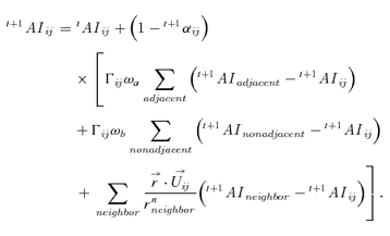
(4)Accident intensity spreading is dominated by two ingredients: “inner factor” and “outer factor.” The dynamics of propagation of the intensity is first controlled by the diffusive effect, which is the inner factor. This implies that intensity flux liberated from the accident epicenter travels outward to the adjoining cells and once each of these incident cells become saturated with the intensity, they in turn begin to act as new intensity sources and the intensity flux begins to diffuse from these cells into their respective neighborhoods. The intensity gradient, which expresses different meanings in different accidents, is the driving force governing this outward propagation of the intensity flux. It means concentration gradient in toxic gas dispersion and temperature gradient in heat spreading and so on. According to common sense, accident spreading is also influenced by some outer factors. For example, wind and terrain slope will affect the distribution of the toxic gas concentration and temperature difference between the ambience and the accident hazards will result in convection. We say that the intensity propagation is also governed by the transporting effect. The dissipative effect is also an important outer factor, which perhaps changes the way of the intensity spreading. While spreading, barriers such as building, river, trees, and sedimentation may all weaken the accident intensity.
Based on above analysis, three common rules can be extracted, i.e., diffusive effect, transporting effect, and dissipative effect, which the accident intensity spreading obeys. Three generalized coefficients are defined to illustrate the three rules:
- 1
Diffusive coefficient (Γ): the ability of intensity spreading from high intensity to low intensity. It is the intrinsic attribute of the accident intensity spreading.
- 2
Transporting coefficient (τ): the ability that environment transports the intensity.
- 3
Dissipative coefficient (α): the ability that outer factors weaken (strengthen) the intensity.
The three general coefficients are critical for simulation results, and they may be functions of other physical quantities in some complex scenarios. They express different meanings in different accidents. For example, the diffusive coefficient expresses gas diffusive coefficient in toxic gas dispersion, while it means thermal energy diffusive coefficient in heat spreading.
 (5)
(5)(1) Diffusive effect rule.
 (6)
(6)(2) Transporting effect rule.
 (7)
(7) are respectively scalar and vector indicating the distance between neighborhood cells and target cell, n is the distance impact factor, and
  is a vector indicating the direction of accident spreading.
(3) Dissipative effect rule.
 (8)
(8) (9)
(9)2.2. Domino Effect Analysis
To study the domino effect, the cells are sorted into two categories, general cells (cellg) and hazardous cells (cellh). General cells are the cells that do not contain the potential hazardous source, and the hazardous cells are the cells that contain the potential hazardous source and serve as potential seed cells. The domino effect is performed through two levels.(15)
At the first level, a screening of all the hazardous cells is done in order to identify hazardous cells and general cells. Then, we need to determine whether certain hazardous cell can cause accidents according to the accident intensity the cell has perceived. For this purpose, three methods have been proposed in the literatures: (1) vulnerability threshold models (the physical effect on the secondary target is higher than a threshold value for damage and then domino effect happens);(19–21) (2) propagation functions based on empirical decay relations for physical effects;(22) (3) propagation functions based on specific probabilistic models.(23,24)
 (10)
(10)2.3. Individual Risk and Aggregated Weighted Risk Analysis
 (11)
(11) (12)
(12)The approach proposed here to treat a sensitive population is based on the assumption that the mean value of intensity fatal to a sensitive population is lower than the mean value of intensity fatal to a normal population, and also that the standard deviation σ of the distribution for a sensitive population is lower than the standard deviation for a normal population. Suitable probit function can be generated for the estimation of individual risk to a sensitive population through adjusting σ and m.(28)
The overall individual risk due to contemporary exposition to different types of physical effects (e.g., a toxic release and a fire, and so on) is also considered. It is calculated as a combination of each related individual risk. The combination can be performed by different strategies. Individual risk is actually probability value; thus probabilistic rules are required for the combination. Four methods have been reported elsewhere.(29) In the approach, one can choose one or several methods to compute the overall individual risk referring to detailed discussions by Cozzani et al. (2005).
 (13)
(13)2.4. Algorithm of the Systematic Approach
An algorithm of the systematic approach has been developed (Fig. 1), where simulation starts at t = 0 and T is the maximum time, user defined. The study area is divided into a two-dimension lattice of cells, and the attributes (hazardous factors, natural factors, and social factors) of each cell are identified. Seed cells that can cause the primary accidents are selected and accident scenarios are developed. The algorithm evaluates the intensity state of each cell in the matrix with respect to the neighborhood cells, taking into account diffusive effect, transporting effect, and dissipative effect. After obtaining the intensity state of each cell, we judge whether some cell contains a potential hazardous source; if yes, we judge whether the intensity of the cell exceeds the threshold; if yes, we take the cell as a seed cell in the next time step. Otherwise, we directly do the next simulation. During each simulation step, we will take population density state and population sensitivity state into consideration. And then, we can get individual risk state in each cell and aggregated weighted risk in a cluster of cells at time t+ 1.
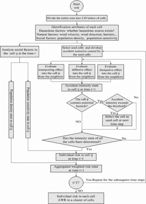
Algorithm of the cellular automata-based systematic risk analysis for emergency response.
The algorithm is run synchronously for every cell present in the lattice. The emerging scenario including domino effect in the subsequent time step is automated. The algorithm is run repeatedly in order to generate the scenarios for all subsequent time steps. This is pursued until the number of time steps becomes larger than the user-defined constant. Consequently, the algorithm is able to generate real-time individual risk and aggregated weighted risk at the end of every time step.
3. APPROACH APPLICATION: AN ILLUSTRATIVE EXAMPLE
3.1. Hypothetical Accident Scenarios
To illustrate the application of the systematic approach, we made simulations on a fictitious city based on THU-CPSR city model, which was designed to simulate a real city with the scale of 5,250 × 4,410 m. There are two commercial buildings, 10 residential buildings, two workshops, three LNG gas containers, and a petrochemical industry in the city. There are river and virescence areas to separate the industrial and residential areas. Therefore, the model can represent a complex city with a cluster of potential hazardous sources and heavy population density. The city model is shown in Fig. 2.
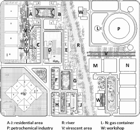
THU-CPSR city model.
The fictitious city is divided into uniform grids of 35 × 35 m. As illustrated in the article, the purpose of the approach proposed here is for risk analysis during emergency response. According to Abrahamsson,(31) the process of risk analysis has a lot of uncertainty and the more detailed spreading simulation might not play a greater role for the results of risk.(31) Therefore, the size of cell needs not be too small. Besides, in our city model, the attribute of each cell is homogeneous when the size is 35 × 35 m. If the size is larger, the attribute of some cells may not be homogeneous. This will bring great trouble for the computations and may affect the precision of the results. Taking the above analysis into consideration, we think that the size (35 × 35 m) is appropriate in our example.
L, M, and N (see Fig. 2) are potential hazardous sources that may cause pool fires. The vulnerable areas are A to J (see Fig. 2), which represent residential areas with heavy population. A hypothetical scenario is used to illustrate the application of the approach. A gasoline leak in one of the gasholders formed a liquid pool at M and flashing of the liquid gasoline results in a pool fire. If the thermal intensity at L and N exceeds the threshold value (10 KW/m2 is used here), derivative pool fires may happen.
During a fire incident, the dominant form of energy that causes maximum damage is the thermal intensity, which propagates via conduction, convection, and radiation. Therefore, accident intensity expresses thermal intensity in this situation. For pool fires, there is an initial unsteady phase in which the burning rate accelerates, a steady state where equilibrium is achieved, and finally a dying down phase in which the accident intensity dissipates to zero. The amount of thermal intensity is influenced by factors such as pool diameter, flame lip effects, the amount of fuels, and so on. In most pool fires, it passes very quickly from unsteady state to steady state.(32,33) Therefore, only the steady state is considered here, and thermal intensity from pool fire is considered to be constant, i.e., 100 KW/m2.
A constant heat value distribution in space would be expected from a pool fire having a constant thermal intensity, but the constant value cannot be achieved as soon as the fire reaches the stable state. It needs time for each cell to achieve the constant state in the steady state. This time is vital for emergency response. If efficient emergency rescue is performed during this time, the loss of life and property may be reduced and a domino effect may also be avoided. In our approach application, the process will be discussed.
3.2. Methods
 (14)
(14) (15)
(15) (16)
(16) .
.Now, we turn to dissipative effect. Unlike in the case of an absolute vacuum, the participating media may attenuate the released thermal intensity due to absorption and scattering. Referring to Section 2, an isotropic effect of barriers is assumed. The dissipative coefficients used here obey the principle that different objects have different dissipative ability. The exact values need to be obtained from experiments.
According to F. P. Lees,(32) the mean value of the intensity fatal to normal population m is 7.775, the standard deviation σ is 0.3903. The individual risk is computed with Equations (11) and (12). The aggregated weighted risk in the residential areas A to J were mainly analyzed. The aggregated weighted risk can be calculated using Equation (13). Table I presents the information about the population density, and the total number of the population of each residential area. We regard population density as constant in the example for simplicity. The combination of site monitoring and a GIS database can be used to obtain the real-time data of population density in practical application.
| Residential Area No. | Population Density (no./km2) | Total Number of Population | Residential Area No. | Population Density (no./km2) | Total Number of Population |
|---|---|---|---|---|---|
| A | 31,020 | 4,484 | F | 17,143 | 1,323 |
| B | 29,388 | 4,132 | G | 4,082 | 1,323 |
| C | 31,020 | 3,648 | H | 14,694 | 1,188 |
| D | 31,020 | 4,750 | I | 14,694 | 1,512 |
| E | 33,469 | 5,248 | J | 14,694 | 1,584 |
3.3. Results and Discussions
The results under homogeneous conditions and heterogeneous conditions were computed to illustrate the CA method's advantage in treating heterogeneous conditions. Here, homogeneous conditions mean that there exist no intercepting objects in all cells (αij = 0). Heterogeneous conditions arise when there are intercepting objects in some cells and the conditions are different in different cells. Domino effect under the two conditions was also analyzed.
Fig. 3 gives the thermal energy varying with time at potential hazardous sources L and N. A significant difference of thermal intensity value can be observed under the two conditions. The thermal intensity under homogeneous conditions is higher than that under heterogeneous conditions at the same time. For example, at t = 600s, the thermal intensity under homogeneous conditions is 5.17 KW/m2 and its counterpart is 3.32 KW/m2 at L. A similar conclusion can be obtained at N, and the two values are 8.84 and 6.61 KW/m2. Due to the impact from the intercepting objects, time to cause derivative accidents is also different and the existence of intercepting objects can delay the time. Under homogeneous conditions, L and N can cause derivative accidents at t = 1005s and t = 697s and the results are 1425 and 975s under heterogeneous conditions.
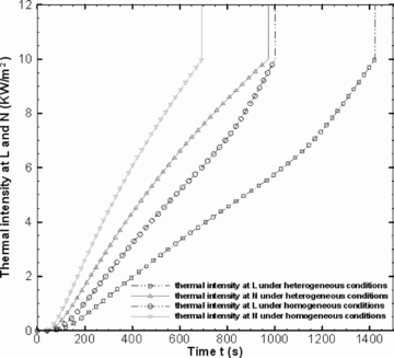
Domino effect analysis. Derivative accident occurs when the thermal intensity at potential hazardous sources (L and N) is not less than 10 KW/m2.
The contours of thermal intensity were also computed (Fig. 4). The results under homogeneous conditions are regular curves, while the impact of heterogeneous conditions on the results can be seen, which makes the curves not smooth and is closer to reality. One can also conclude that designing isolated areas to separate an industry area and a residential area, and different industry areas is advantageous to reduce accident impact and prevent domino effect. Comparing the two groups of figures, one can see that the existence of river and virescence areas greatly reduces the thermal intensity. For example, in the area G thermal intensity has been more than 10 KW/m2 without intercepting objects, but under heterogeneous conditions the value is less than 10 KW/m2 at t = 800s (Figs. 4(C) and 4(D)). At t = 800s, thermal intensity at N is over 10 KW/m2 and a secondary accident has happened under homogeneous conditions (Fig. 4(D)). Due to the absorption of buildings, the intensity is less than 10 KW/m2 at L and no secondary accident happened at t = 800s (Fig. 4(C)). The potential hazardous source L received nearly 10 KW/m2 thermal intensity at 1000s (Fig. 4(F)), and the tertiary accident will occur soon, while the counterpart intensity is only about 5 KW/m2 (Fig. 4(E)), which cannot cause any derivative accident. Besides, according to the results, one can determine emergency rescue time. At t = 975s, the secondary accident occurs at N. So if emergency rescue power is sent to N during this time, a secondary accident may be prevented. If not, at least one can delay the time of the secondary happening to obtain more time for people evacuation.
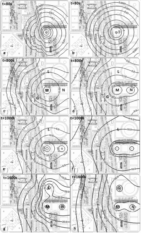
Contours of thermal intensity under two conditions at different times. At t = 0, the accident happened at M. Figs. A, C, E, and G represents the results under heterogeneous conditions and Figs. B, D, F, and H represents the results under homogeneous conditions.
Individual risk is analyzed and the simulation results of individual risk contours are discussed (Fig. 5). From contours of individual risk, one can obtain the real-time information about the distribution of individual risk. As expected, for an emergency manager, individual risk is much more practical than accident intensity during emergency response. For example, at t = 800s (Fig. 5(B)), although the thermal intensity in most of the residential areas is more than 1 KW/m2, the individual risk is much less than 1 × 10⁻⁶. Therefore, the manager can easily judge that at this time most of the residential areas are safe (we think that individual risk less than 1×10⁻⁶ is safe). At t = 1200s (Fig. 5(C)), the individual risk around building G is more than 1 × 10⁻⁶, and the area is not safe anymore. With time going by, the unsafe area expands gradually. At t = 2600 s (Fig. 5(D)), almost all residential buildings are in danger except building A. Besides, according to the contours of individual risk, emergency managers can issue prewarning information to guide the people to evacuate. If one neglects tertiary accidents, it is a good strategy to guide people to evacuate to the northwest area. However, a high risk source L exists in the north and it will cause an accident at t = 1425s. Comprehensively considering these factors, a west side evacuation is strongly recommended (Figs. 5(E) and 5(F)).
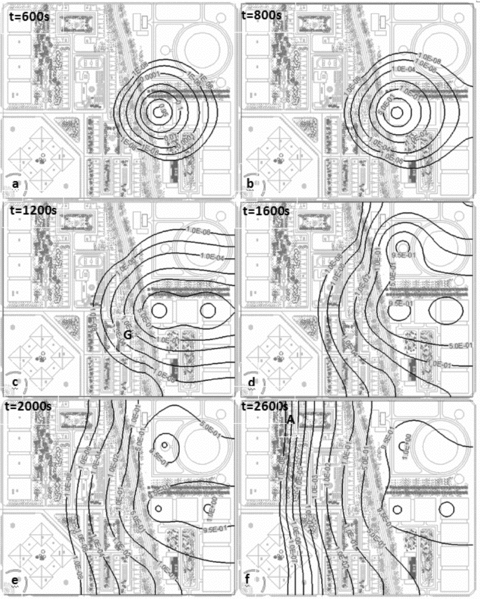
Contours of individual risk under heterogeneous conditions at different times. At t = 0, the accident happened at M.
Aggregated weighted risks in the 10 residential areas were also computed at different time. The results are given in Table II. Some significant conclusions can be obtained to help emergency managers allocate emergency rescue resources. For example, the AWR is very low in all the 10 areas at t = 600s and t = 800s. At t = 1200s and t = 1600s, the AWR at area E, G, and J is much higher than that at other areas, especially area G where the AWR is the highest. At t = 2000s, the area E is the most dangerous area. After t = 2000s, nearly all areas have high AWR. Based on above analysis, the following resources allocation strategy is advised: (1) at the first half an hour of emergency response, more rescue resources should be sent to E, G, and J; (2) after that, D, F, H, and I gradually need more resources.
 |
600s | 800s | 1200s | 1600s | 2000s | 2600s |
|---|---|---|---|---|---|---|
| A | 0.00000000 | 0.00000000 | 0.00000000 | 0.00000000 | 0.00000000 | 0.05801328 |
| B | 0.00000000 | 0.00000000 | 0.00000000 | 0.00000000 | 0.03297678 | 70.69564293 |
| C | 0.00000000 | 0.00000000 | 0.00000000 | 0.00000000 | 0.00007334 | 0.45263844 |
| D | 0.00000000 | 0.00000000 | 0.00000102 | 0.00110798 | 0.20017541 | 34.11987993 |
| E | 0.00000238 | 0.00072004 | 0.18783947 | 4.60474650 | 98.56040847 | 1126.08295703 |
| F | 0.00000000 | 0.00000000 | 0.00008104 | 0.01595472 | 0.70950394 | 27.93128237 |
| G | 0.00462710 | 0.07861287 | 1.46759059 | 9.16648734 | 35.34787203 | 115.56288804 |
| H | 0.00000000 | 0.00000000 | 0.00000000 | 0.00007405 | 0.01880954 | 3.57464209 |
| I | 0.00000000 | 0.00000000 | 0.00005910 | 0.02229424 | 1.22450960 | 46.84007340 |
| J | 0.00000000 | 0.00001079 | 0.01515049 | 1.31135140 | 24.86859071 | 316.95609140 |
4. CONCLUSIONS
Emergency response is applying science, technology, planning, and management to deal with extreme events. Developing a meaningful model capable of conducting emergency response is an arduous task that requires the contributions of many individuals from several disciplines. The cellular automata-based systematic risk analysis approach for emergency response presented here is a preliminary attempt to contribute to the gigantic efforts.
In this article, three cellular automata transition rules, which work through diffusion, transport, and dissipation mechanism, are proposed. The approach can take multiple factors into account such as physical and social characteristics of the site and can also handle domino accidents. As an outcome, two risk indices are proposed to assist emergency managers to make decisions. The potential application of the proposed approach for risk analysis and emergency response has been illustrated with an example. The results demonstrate that the CA method can easily treat heterogeneous conditions, and give an irregular shape of the area of impact of an accident, which is much more realistic assessment for risk analysis. Besides, according to the results, we conclude that individual risk is useful to plan evacuation strategies and aggregated weighted risk can help emergency managers to allocate rescue resources rationally and optimize emergency response programs.
In reality, before the approach is brought to bear on any complex problems, there are three issues meriting special attention. First and foremost, it must be emphasized that cellular automaton is a computational tool, whose effectiveness depends upon its accurate calibration on the basis of data from experimental results as well as those from past accident histories. Research in these areas has been continuing across the world but needs greater impetus. Besides, discussion of the size of the cells is also needed according to real problems in the future research. Secondly, the process of emergency response is very complicated, and some other social factors may also affect the results of risk assessment, such as important facility density, transportation system density, rescue power distribution, and so on. The detailed discussion of those factors should be conducted in future research. Last but not least, the merit of the approach should be judged in real-life scenarios, although it is hard. It is a good way to validate and improve the approach in future emergency response drills. The data gathered from real cases are also meaningful for this purpose.


