GINI DECOMPOSITION AND GINI INCOME ELASTICITY UNDER INCOME VARIABILITY
ABSTRACT
The Gini income elasticity has been used to assess the impact of marginal proportional changes in income from a given source on inequality in total income. This note extends the methodology to take into account income variability.
I. INTRODUCTION
The Gini Income Elasticity (GIE hereafter) is a parameter that measures the impact on the (extended) Gini index of income inequality of a marginal proportional change in an income source (e.g., Lerman and Yitzhaki, 1985; Stark et al., 1986). Estimates of the GIE have been used, among others, for assessing the impact on inequality of increases in outlays for social programs (e.g., Lerman and Yitzhaki, 1994; Wodon and Yitzhaki, 2002). However, while an increase in funding for programs such as unemployment benefits may reduce inequality in mean income, it may also reduce income variability or risk, and this is not taken into account in the traditional decomposition of the Gini index. In this note, we show that under income variability (assuming that the observations represent a draw from states of nature), an income source has three GIEs corresponding to the three ways in which the income source affects the certainty equivalent income: (i) the mean income from the source over time, (ii) the variability in income from the source and (iii) the correlation over time between income from the source and income from other sources. The total impact on inequality of a marginal change in income from the source is then a function of these three GIEs.
II. METHOD
 (1)
(1) (2)
(2) (3)
(3) (4)
(4) does not represent the Bernoulli utility function of the individual, but rather a social judgement on the impact of income variability on welfare. Denote by μi the individual's mean income over time. The cost of variability,
  , is defined by
 (5)
(5) (6)
(6) is the Arrow–Pratt absolute risk aversion index measured at μi, and
  is the variance of the individual's income. In this note, for simplicity, we assume that the social planner has a normative evaluation of risk aversion. This normative evaluation is represented by a constant absolute risk aversion (denoted by ρ), so that
 (7)
(7) (8)
(8) (9)
(9) is the covariance between a and b. We have
 (10)
(10) . Using (8)–(10), (7) may be rewritten as
 (11)
(11) is the cost of the income variability of source j, and
  is the cost (or benefit) due to the covariance between source j and other income sources. If we denote by
  and
and  the mean values over the population as a whole of μij, φij and ξij, and as before by m the mean value of yi, applying (1)–(11) yields for each income source three components in the decomposition of the Gini

 (12)
(12) (13)
(13) (14)
(14)
With cross-section data, since we do not observe income variability, only the first term on the right-hand side of (14) appears, so that whether an income source increases or decreases inequality at the margin is solely determined by whether the GIE  is above or below one. In a panel setting, we have instead three sources of impact at the margin, and thereby three GIEs related to (i) the mean income from the source over time, (ii) the variability of the source, and (iii) the correlation between the source and other sources over time. For example, a source such as unemployment benefits may reduce inequality in certainty equivalent income at the margin not only through targeting individuals with comparatively low mean income, but also through reducing income variability for these individuals, with this beneficial effect appearing through the third GIE in (14).
 (15)
(15) (16)
(16) (17)
(17) and
and  are defined analogously. Following a small proportional change in income from a source, we will have


III. CONCLUSION
Most of the work for assessing the impact of public transfers on inequality is based on cross-sectional data. Yet many transfers are designed not only to reach the poor, but also to offset the impact of income variability on welfare and on vulnerability. In this note, we have extended the source decomposition of the Gini index of inequality to show how to evaluate the impact at the margin on inequality of a proportional increase in program outlays under income variability. When considering inequality in certainty equivalent income, each income source can be said to have three Gini Income Elasticities corresponding to the three terms appearing in the Taylor approximation of the individual's certainty equivalent income, namely the mean income from the source, the variability of the source over time, and the covariance between the source and other income sources over time. The importance of such sources of variability remains an empirical matter that goes beyond the scope of this note.
The Gini coefficient has a unique underlying social welfare function that is based on the rank of individuals. In future research it would be interesting to propose a more general framework to account for income variability. This will be in line with the work of Makdissi and Wodon (2002), Duclos et al. (2005, 2008) and Makdissi and Mussard (2008a,b) who propose more general frameworks to analyse tax and transfer reforms for all social welfare function that obey Fishburn and Willig (1984) generalized transfer principles.
Footnotes
Appendix
APPENDIX: PROOF OF EQUATION (13)
 ((A.1))
 is defined analogously. However,
 ((A.2))
 ((A.3))
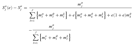
 ((A.4))
 and
and  have analogous forms. For j = k,
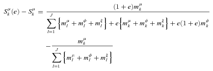
 ((A.5))
 has an analogous form. However
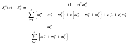
 ((A.6))
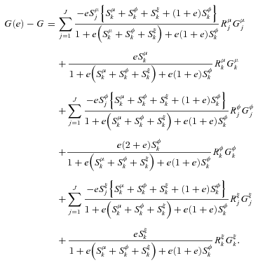
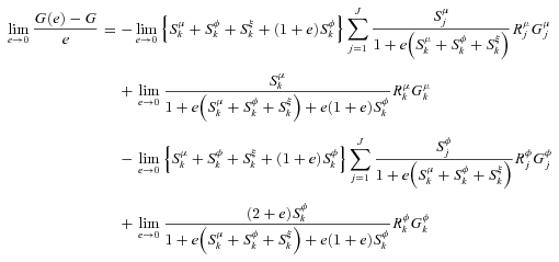

 ((A.7))
It is straightforward to get (13) from (A.7). The proof for the extended Gini index is similar.


