Latitudinal gradient of taxonomic richness: combined outcome of temperature and geographic mid-domains effects?
Gradients latitudinaux de richesse taxonomique: résultat combiné des effets de milieu de domaine géographique et thermique?
Abstract
enFor several decades, the origin and ecological consequences of large-scale continental and marine Latitudinal Gradients of Taxonomic Richness (LGTR) have been intensively debated. Among the various hypotheses, it has been proposed that a LGTR is the by-product of a geographic mid-domain effect, i.e. the result of a random distribution of ranges of taxa between physical hard boundaries such as the continent/ocean interface. In order to more realistically evaluate the role of the mid-domain effect on the origin and evolution of the LGTR of marine planktonic organisms, we present a 2D model based on a cellular-automaton approach in which sea surface temperatures (SST) and currents are forced in the biogeographic dispersal of a randomly generated clade (a 2D ‘geophyletic’ model). Sensitivity experiments allow to evaluate the effects of currents, SST and the geographical origin of a clade on the formation and shape of a LGTR for planktonic organisms when coupled with a geographic mid-domain effect. Results are discussed in the light of the empirical LGTR of extant planktonic Foraminifera in the Atlantic Ocean. Independently of any other biotic or abiotic parameter, inclusive of the surface currents and origination/extinction absolute and relative rates, our simulations show that the coupling of the mid-domain effect with two critical parameters, namely the shape and intensity of the SST gradient and the geographic origin of a clade, produces realistic patterns of diversity when compared with the observed LGTR of extant atlantic planktonic foraminifera. The results illustrate a non-linear relation between a unimodal latitudinal SST gradient and a resulting bimodal LGTR characterized by a drop in species richness near the equator. This relation indicates that the SST gradient exerts a mid-domain effect on the LGTR. The latitudinal positions of the modal values of the LGTR are also found to be influenced by the geographic origin of the simulated clade.
Résumé
frDepuis plusieurs décennies, l'origine et l'interprétation écologique des Gradients Latitudinaux de Richesse Taxonomique (LGTR) marins ou continentaux, ont été intensivement débattues. Parmi de nombreuses hypothèses, il a été proposé qu'un LGTR puisse être le sous-produit d'un effet de milieu de domaine géographique, i.e. le résultat d'une distribution aléatoire des répartitions des taxa entre deux limites physiques telles que l'interface continent/océan. Afin d’évaluer plus efficacement le rôle de cet effet sur l’origine et l’évolution des LGTR des organismes planctoniques marins, nous proposons un modèle 2D basé sur une approche de type automate cellulaire dans laquelle les températures des eaux de surface (SST) et les courants régulent la dispersion biogéographique d'une phylogénie générée aléatoirement (un modèle «géophylétique»). Ce modèle permet d’évaluer les effets des courants, des SST et de la dépendance thermique des espèces sur la mise en place et la forme d'un LGTR impliquant des organismes planctoniques. Il permet aussi de discuter des influences respectives de ces paramètres quand ils sont superposés à l'effet de milieu de domaine géographique. Les résultats sont discutés à partir du LGTR empirique des foraminifères planctoniques atlantiques actuels. Indépendamment de tout autre paramètre biotique ou abiotique, y compris les courants ainsi que les taux relatifs et absolus d'apparition et d'extinction, les simulations font apparaître que le couplage de l'effet de milieu de domaine à deux contraintes principales, la forme et l'intensité du gradient de SST ainsi que la localisation géographique de l'origine du clade, produit des représentations réalistes de la diversité comparées au LGTR observé pour les foraminifères planctoniques actuels de l'océan atlantique. Nos résultats indiquent une relation non-linéaire entre la structure globale d'un gradient unimodal de SST et le LGTR bimodal correspondant, montrant une baisse de richesse spécifique au niveau de l’équateur. Cette relation suggère que le gradient de SST exerce un effet de milieu de domaine thermique sur le LGTR. Les positions latitudinales des modes du LGTR sont aussi influencées par le lieu d'origine du clade simulé.
Introduction
The latitudinal gradient of taxonomic richness (LGTR) is one of the most studied patterns of global biodiversity (e.g. Dobzhansky 1950; MacArthur 1965; Stehli et al. 1969; Currie and Paquin 1987; Gaston 2000; Hillebrand 2004). It is known to occur in a majority of taxonomic groups and is manifested in most cases as a decreasing number of taxa (species, genera or families) from low to high latitudes: tropical areas show higher taxonomic richness values than at the poles. The latitudinal diversity cline recognized on land and sea is classically described as unimodal with a taxonomic richness monotonically increasing from the pole to the equator (e.g. Pianka 1966; Gaston 2000). However, a second pattern has to be considered. It is often found in marine environments and consists of a bimodal gradient of taxonomic richness with two maxima centred near the Tropics of Cancer and Capricorn, separated by a drop of taxonomic richness near the equator (e.g. Rutherford et al. 1999). This bimodal pattern is usually interpreted as being a derivative from a primarily unimodal richness gradient.
Classical explanations
Although many ecologists, biogeographers and biologists have discussed the ecological and evolutionary mechanisms at the origin of LGTR (see Rohde 1992 and Willig et al. 2003 for a review of the different classical factors), hypotheses explaining the spatial structure and temporal variability of the distribution of taxonomic richness on Earth are still contentious (e.g. Clarke 1992; Chown and Gaston 2000).
Indeed, about 30 possible explanations have been proposed to explain the origin of the LGTR. Most of them imply empirical, direct or indirect relationships between taxonomic richness and climatic gradients. These involve, e.g. potential evapotranspiration (Currie and Paquin 1987), temperature (Turner et al. 1987), productivity (Kaspari et al. 2000), which are all grouped within the energy-hypothesis (Currie 1991). Other explanations imply evolutionary and dispersal rates (e.g. Pianka 1966; Graham et al. 1996; Wilson 1998). Some of the determinants of the formation of the LGTR can also involve parameters such as area, predation and competition levels, or biotic spatial heterogeneity. It has been shown that the majority of these hypotheses cannot be used for the purpose of a general or unique explanation; moreover, most of them contain various degrees of circularity or are not supported by sufficient evidence (Rohde 1992). Considered separately, each of these appears insufficient to fully explain the existence of the LGTR as observed on land and sea. Furthermore, most of these hypotheses do not take into account the phylogenetic time dimension, i.e. the deep-time scale at which species originate, evolve, and become extinct.
The mid-domain effect
Biodiversity and geometric constraints
Recently, all of these hypotheses were reduced to five main explanations grouped in the following classes: energy availability, habitat heterogeneity, evolutionary time, area, and geometric constraints (Rahbek and Graves 2001; Whittaker et al. 2001). Among these five classes, the geometric constraints hypothesis is particularly worthy of attention because of the probabilistic nature of its explanatory principle. In the absence of any deterministic environmental or historical gradients, the formation of a latitudinal, longitudinal, altitudinal or depth gradient of taxonomic richness might be the direct and single consequence of the random spatial distribution and overlap of the ranges of taxa. Under these conditions, the random placement (in one or two dimensions) of species geographic ranges on a bounded domain (e.g. sea, continent, island, mountain) never generates a uniform spatial distribution, but always produces a peak of taxonomic richness near the centre of the area: the ‘mid-domain effect’ (Colwell and Hurtt 1994; Ney-Nifle and Mangel 1999; Colwell and Lees 2000; Jetz and Rahbek 2001; Grytnes and Vetaas 2002; McCain 2003, 2004; Colwell et al. 2004). Following this hypothesis, the latitudinal, longitudinal, altitudinal or bathymetric positions of the species ranges directly determine the shape of the taxonomic gradient.
Evaluation of the mid-domain effect in biogeographic patterns
Earlier 1D simulations with geometrically constraining boundaries (Colwell and Hurtt 1994; Colwell and Lees 2000) showed that a LGTR can be the simple geometric by-product (the mid-domain effect result) of the random distribution of taxa ranges between ‘hard’ boundaries (e.g. coast lines), and that a LGTR does not necessarily require any biotic and/or abiotic deterministic explanation. This result can be applied to any living organism and any particular biogeographic setting. An LGTR emerges even if no deterministic environmental gradient is applied in the simulation. By producing a mid-domain effect, this null geometric model suggests that an observed LGTR can simply be the result of chance: between two fixed boundaries, randomly distributed ranges always give rise to a peak or a plateau of taxonomic richness (Lees et al. 1999; Jetz and Rahbek 2001). Thus, the random location of ranges between fixed geographic boundaries may generate distributions of taxonomic richness comparable with empirical distributions.
Several of the documented past or present taxonomic richness gradients present, at first approximation in both hemispheres, a parabolic-shape with a maximum value at middle or low latitudes (McCoy and Connor 1980; Turner 1981; France 1992; Angel 1993; Crow 1993; Brown and Lomolino 1998; Willig and Lyons 1998; Crame 2000, 2001, 2002; Culver and Buzas 2000; Sax 2001; Ellison 2002; Connolly et al. 2003; Shen and Shi 2004), intermediate altitudes (Rahbek 1995, 1997; Fleishman et al. 1998; Kessler 2001; Lomolino 2001; Grytnes and Vetaas 2002; Sanders 2002; Grytnes 2003; Bhattarai et al. 2004; McCain 2004) or intermediate marine depths (Rex 1981; Paterson and Lambshead 1995; Pineda and Caswell 1998; Smith and Brown 2002). For instance, the distribution of many Madagascan insect species and the resulting, dome-shaped LGTR with a modal value at mid-latitudes and elevations, are less in agreement with climatic variables than with the prediction of the geometric mid-domain model (Lees et al. 1999). It has also been documented that species richness of ant communities peaks at mid-elevations, suggesting that the mid-domain effect could also have an important part in the development of altitudinal gradients (Sanders 2002; McCain 2004).
Nevertheless, the geometric model has generally a poor explanatory power, especially when applied to 2D cases and has been heavily criticized (Bokma et al. 2001; Koleff and Gaston 2001; Hawkins and Diniz-Filho 2002; Laurie and Silander 2002; Valle de Britto Rangel and Diniz-Filho 2003; Zapata et al. 2003; see Colwell et al. 2004 for a discussion of the concept and applications of the mid-domain effect). Possible errors in sampling or interpolation of the number of taxa can also explain some of the discrepancies between the output of geometric models and observed LGTR (e.g. Colwell and Hurtt 1994; Rahbek 1995; Grytnes and Vetaas 2002). Problems inherent to the construction of the geometric models can also arise as most of the previous tests of geometric null models versus observed data did not factor in an environmental or historical component. This addition may adjust the output of geometric models and observed LGTR. For instance, it is often considered that the dispersion limits of a taxon could be deterministically controlled in low latitudes/altitudes by the increase of severe biotic conditions like competition or predation (Kaufman 1995; Brown et al. 1996; Sax 2001). Furthermore, it is generally suggested that severe abiotic conditions at high latitudes/altitudes (e.g. frequent climatic variations and/or extremely low-temperatures) could induce natural boundaries for the ranges of many organisms. Consequently, geometric models with a random placement of the ranges of species should be combined with environmental parameters in order to more realistically predict observed LGTR.
In order to better understand the consequences of the omission of the environmental gradients and the phylogenetic time dimension in the construction of geometric models, we introduce here a more general, cellular automaton-type, 2D geometric model based on a step-by-step simulation and constrained biogeographic dispersal of a random phylogeny – a ‘geophyletic’ model. Results of the simulations are illustrated in the particular biogeographic, thermal and ocean currents configuration of the present-day North and South Atlantic. They are discussed in the light of the well-documented present latitudinal gradient of species richness of planktonic Foraminifera (Hemleben et al. 1989; Hilbrecht 1996; Arnold and Parker 1999; Rutherford et al. 1999). Our approach evaluates the effects of currents, sea surface temperatures (SST), speciation and extinction rates, as well as species thermal dependence on the formation and shape of a species richness gradient for planktonic organisms. We also discuss the respective influence of these parameters in combination with a possible geographic mid-domain effect. This work is a first step toward the biogeographic modelling and evaluation of climatic influences in the recovery of marine organisms after mass extinctions (Brayard et al. 2004).
Materials and Methods
The studied bounded geographic area
The model is based on three 120 × 120 matrices representing the Atlantic Ocean and its bordering continents (North and South America, Europe and Africa). Each cell represents one square degree between 100°W and 20°E (continent boundaries), and 60°N and 60°S (latitudinal proxies of the weakening of the SST gradient). The three matrices are: (1) The biogeographic matrix, where the presence or absence of each simulated taxon (hereafter, species) in each sea cell is recorded (as we focus on planktonic organisms, continental cells are obviously ‘non-colonisable’). (2) The sea surface temperatures matrix (data from the National Oceanic and Atmospheric Administration, Fig. 1a). (3) The sea surface currents (SSC) matrix, with directions and intensities based on the present Atlantic surface currents (data from Pickard and Emery 1990; Fig. 1b). Because the map represents a non-iso-surface, a correction-factor (varying with latitude) is applied so that the amount of displacement of each species during one time iteration is kept latitude-independent.
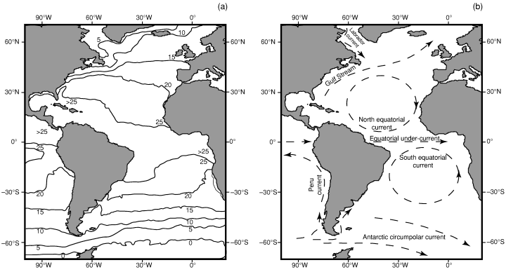
Atlantic Ocean (a) SST (data from the National Oceanic and Atmospheric Administration) and (b) generalized surface circulation (data from Pickard and Emery 1990)
General concept of the ‘geophyletic’ model
Our algorithm consists of a step-by-step generation of a random clade (i.e. a monophyletic assemblage of taxa, using a simple standard Markovian procedure) and its geographic dispersion (sensuRosen 1992 and Cecca 2002) under the direct control of the SST and SSC matrices. It stands in contrast with the classic ‘MBL’ algorithm (Raup et al. 1973; Raup and Gould 1974; Gould et al. 1977; Raup 1977; Stanley et al. 1981) in that it simultaneously controls the growth of the random clade at the local (i.e. cell) level and at the global level. The local geographic control on the evolutionary dynamic of the clade generates ecologically more realistic null models of phylogenesis and community assembly evolution (Hubbell 2001; Webb et al. 2003). Actually, our ‘geophyletic’ model can be described as being globally time-homogeneous in that species origination and extinction probabilities are statistically constant at the global clade level. It is also locally time-inhomogeneous in that local extinction probability is kept species richness-dependent in order to avoid ecologically unrealistic overcrowding of species in local communities. Our model thus combines characteristics of the two main options of the MBL model (‘Damped-Equilibrium’ and ‘Freely Floating’) described by Gould et al. (1977; see Raup 1985).
Inheritance rule of the thermal ranges between mother and daughter species is set as follows: the thermal range of the daughter species must include the temperature of the cell where speciation occurred (extrinsic, physical constraint; Fig. 2). Consequently, the thermal ranges of a mother and a daughter species at least partly intersect (intrinsic, phylogenetic constraint). The effects of this partial constraint imposed on the random evolution of the species thermal range throughout speciation events compare with the Markovian Drift Coefficient used by MacLeod (2002). It is worth noting that in no way is this inheritance process a type of selection controlling the simulation, the thermal range of the daughter species being free to assume many values of the ancestral thermal range. The choice to add this constraint to the model is supported by the observed latitudinal overlap in distributions of closely related planktonic foraminifera (de Vargas et al. 2001).
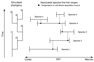
Illustration of the inheritance rule of the thermal ranges between mother and daughter species
The amplitude of each thermal range can be either fixed or randomly chosen from 5°C to 15°C to cover the vast majority of observed distributions of planktonic organisms. Uniform or non-uniform probability functions can be selected for the sorting of thermal ranges. For instance, higher probabilities of random sorting were chosen and assigned to the thermal ranges comprised between 10 and 15 °C in order to more realistically reflect observed distributions of planktonic Foraminifera. Indeed, most planktonic Foraminifera are restricted to portions of the SST gradient such as the tropics, the temperate or the high latitudes, each of these portions spanning temperature ranges of about 10–15°C (Hemleben et al. 1989; Arnold and Parker 1999). This choice of thermal ranges is also in agreement with the temperatures of foraminifer cultures (Bijma et al. 1990).
The amplitude of each thermal range is converted to a 2D geographic range located between 60°N and 60°S. A simulated species can have its geographic range overlapping part of the northern and/or southern hemisphere, or covering the equatorial region. Geometric spatial constraints operate between continent boundaries and the approximate limit of weakening of the SST gradient (near 60°N and 60°S in the Atlantic Ocean). Thus, a geometrical mid-domain effect is expected within this bounded domain, with a near-equatorial peak of diversity. During the simulations, each simulated species can move independently from others (ecological associations of species are deliberately ignored in order to generate the ‘geophyletic’ null model), under the limiting controls of SST and SSC matrices.
Procedure steps of the algorithm
Each time-iteration of the algorithm can be divided into five steps, where the controlling parameters of the simulation are tested consecutively for each filled cell of the biogeographic matrix (Fig. 3). (1) Speciation: a new species can originate in any cell filled by the mother-species, given a probability of speciation inversely correlated with the number of neighbouring cells occupied by the mother-species. Changes in speciation rates during the simulation are allowed. (2) Species displacement: a species occurring in a cell can move into any other randomly chosen adjacent cell, provided that it is not already present in that new cell and that the temperature of the new cell is compatible with its own thermal range. The SSC matrix directly controls the probability distribution for each cell and each species. The probability of dispersion can be adjusted to correspond to the intensity of the surface currents (accelerating or slowing down the propagation of the species). Consequently, each species is let free to colonize part or all of the geographic area compatible with its thermal range. (3) Extinction: two cases with distinct associated probabilities, ‘local’ and ‘complete’ extinctions, are distinguished and treated separately. The disappearance of a given species in one cell (‘local’ extinction) does not affect the neighbouring cells occupied by the same species. In the case of a ‘complete’ extinction, all the cells filled by the species are simultaneously emptied. As for the speciation rates, both ‘local’ and ‘complete’ extinction rates can be modified during the simulation. (4) Diversity threshold of cells (i.e. carrying capacity): in order to avoid ecologically unrealistic accumulations of species in cells, ‘local’ extinctions are randomly generated (i.e. the probability of ‘local’ extinction is deterministically increased) in cells where the number of species is greater than a given threshold saturation value. This threshold determines the number of species supported by the environment. The default value is arbitrarily fixed at 30 species, a value based on the observed maximum association of co-existing species of Atlantic planktonic Foraminifera (Rutherford et al. 1999). (5) Finally, the species richness is calculated for each cell of the biogeographic matrix as the sum of co-occurring species. Even if these four first steps are successively executed for each filled cell at each time iteration, the speciation, extinction and displacement events may not necessarily occur, thus making the changes in species richness of a given cell independent from those of other cells.
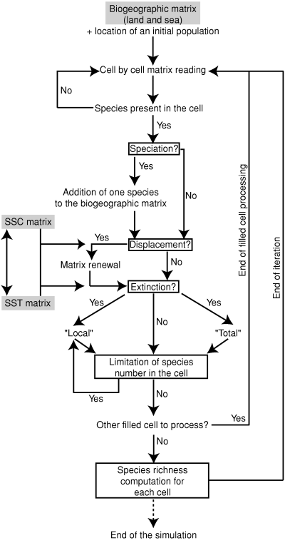
Flow chart of the 2D ‘geophyletic’ model. See text for details about the different tests and procedures contained in each step
Therefore, running our ‘geophyletic’ model for several hundreds of iterations (depending on the selected speciation and extinction rates) allows us to construct theoretical patterns of species richness distribution under the SST and SSC-constrained hypothesis of random evolution and geographic dispersal. Such theoretical patterns of species distribution can thus be compared with observed distribution patterns. Under given observed SST and SSC conditions, differences between simulated and observed patterns would imply departure from the null hypothesis of random evolution as generated by the model. For instance, such differences may result from non-random spatio-temporal fluctuations of speciation and extinction rates, as asserted by some ‘evolutionary-time’ hypotheses (Pianka 1966; Rahbek and Graves 2001; Whittaker et al. 2001). Such differences could also result from non-random geographic dispersion of species, as directly or indirectly asserted by some ‘energy availability’, ‘habitat heterogeneity’ and ‘area’ families hypotheses.
Results
Patterns of latitudinal species richness
We ran our ‘geophyletic’ model, constrained by modern Atlantic SST and SSC conditions, using the following speciation and extinction probability values: allopatric speciation = 5 × 10⁻⁶, parapatric speciation = 2 × 10⁻⁶, sympatric speciation = 1 × 10⁻⁶, ‘local’ extinction = 1 × 10⁻², and ‘total’ extinction = 1 × 10⁻⁴ (it must be here again stressed that speciation and ‘local’ extinction are controlled at the local, one square degree cell level). With such parameter values, the simulations reached a stable dynamic equilibrium after c. 1000 iterations. The results presented and discussed hereafter were obtained from 1200 iterations; several independent simulations (initiated with distinct, randomly chosen uniform pseudo-random number generator seeds) yielded very similar patterns of diversity indicating that the model had reached equilibrium.
Given the assumption of an inter-tropical geographic origin of the clade, we simulated the distribution of species richness and its corresponding LGTR for planktonic organisms (Fig. 4, to be compared with Fig. 5a). Contrary to the classic expectation of monotonically increasing species richness from the pole to the equator (unimodal LGTR from pole-to-pole), the simulated distributions and gradients clearly show two peaks of maximum species richness centred near the Tropics of Cancer and Capricorn, separated by a marked drop around the equator (bimodal LGTR).
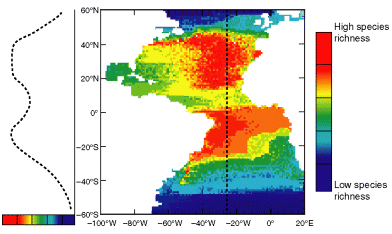
Pattern of distribution of planktonic species richness and associated LGTR simulated with present-day SST and SSC data, randomly generated 10–15°C thermal ranges, a low latitude last common ancestor and no latitudinal gradients of origination and extinction rates (see text for details)
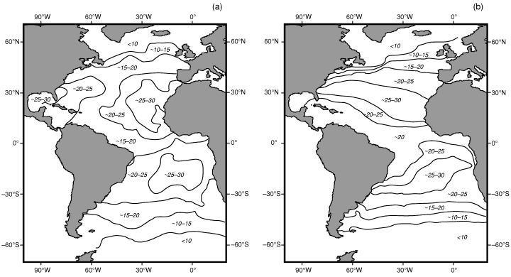
Present-day (a) and predicted (b) planktonic foraminiferal diversity in the Atlantic (adapted from Rutherford et al. 1999)
The shape of the LGTR observed for extant Foraminifera is very similar to that simulated by the ‘geophyletic’ model, with a marked drop of species richness near the equator and highest diversities occurring at the same tropical latitudes (∼15° to 30° in each hemisphere). Our results are close to the pattern predicted by Rutherford et al. (1999; Fig. 5b) on the single basis of the observed polynomial relation between SST and species richness. Even if our results correctly reproduce, both qualitatively and quantitatively, the observed diversity pattern of Atlantic planktonic Foraminifera at a global scale, some minor differences between the simulated and observed diversity patterns exist, notably on the longitudinal location of the maxima of species richness. In the southern hemisphere, the maxima of species richness are shifted toward the west in our simulations. Another discrepancy is the absence of a diversity peak within the Caribbean Sea.
Influential parameters
In order to test the stability and reproducibility of the results, we performed sensitivity experiments by successively varying the parameters controlling the simulations.
The sea surface temperature latitudinal gradient
We first examined the impact of the unimodal pole-to-pole latitudinal gradient of SST on the simulation results. Its intensity has a strong influence on the simulated LGTR: the steeper the SST gradient, the more bimodal the shape of the LGTR. Consequently, the simulated LGTR is unimodaly centred on the equator only for very weak SST gradients. Our simulations, therefore, suggest that the SST gradient is a crucial physical parameter controlling the emergence and shape of the LGTR.
In most of our simulations, the non-linear relation between the simulated bimodal LGTR and SST values is best fit with a third-order polynomial (associated determination coefficient R2 comprised between 0.85 and 0.95), which allows a faithful description of the simulated decreasing richness centred on the equator (Fig. 6). Graphical investigation of the simulated SST/LGTR relationship for various sets of controlling parameters suggests that the inferred third-order polynomial distribution can satisfactorily be divided into three distinct linear segments, which can be isolated by linear Piecewise Analysis (Neter et al. 1990; Toms and Lesperance 2003). For simulations based on the present Atlantic thermal conditions, and independent of the values of other parameters, SST values display two remarkably stable slope changes in the SST/LGTR relation. The first slope change is situated at c. 10°C and the second is found at c. 22–24°C. The first middle/high-latitudes segment is always associated with low values of species richness and corresponds to a low or nil increase of species richness with temperature. The second middle/low-latitudes segment corresponds to a marked increase of species richness with temperature. The third segment (inter-tropical latitudes) corresponds to a significant decrease of species richness with temperature. The location of the thermal breakdown around 22–24°C is also observed by Rutherford et al. (1999: Fig. 3). The breakdown at c. 10°C is also documented in empirical data but is less pronounced. This convergence between the observed and simulated SST/LGTR relationship suggests that our ‘geophyletic’ model generates realistic patterns of diversity.
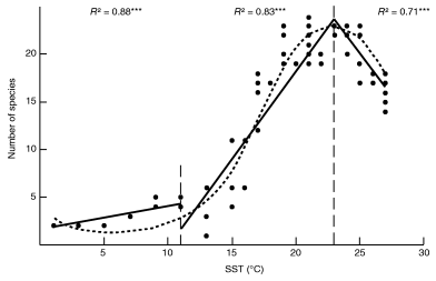
Third-order polynomial and Piecewise analysis of the SST-LGTR relation corresponding to Fig. 4
Amplitude of the thermal ranges of the simulated species
This biological parameter does not affect the bimodal structure of the simulated LGTR but strongly controls its shape. For a given set of simulation parameters yielding a bimodal LGTR, randomly generated broad thermal ranges yield a relatively flattened, but always bimodal LGTR, while narrow thermal ranges yield a relatively steep bimodal LGTR with modal values slightly closer to the equator.
Intensities of the SSC
Although SSC have a strong influence on the timing and local modalities of the dispersion of simulated species, they have no influence on the shape and magnitude of the simulated LGTR. Even in the extreme and unrealistic case where no SSC are imposed in the model, a bimodal LGTR centred on the Tropics of Cancer and Capricorn persists.
Geographic origin of the simulated clade
The geographic origin of the clade has an unexpected effect on the simulated LGTR: the lower the latitude of origination of a clade, the closer the two modal values of the simulated bimodal LGTR. A simulated bimodal LGTR centred on the Tropics of Cancer and Capricorn will result from a tropical last common ancestor. A simulated bimodal LGTR with modes placed at higher latitudes will be generated by a mid- or high-latitudes last common ancestor. This result does not appear to be an artefact illustrating non-equilibrated simulation outputs: it was observed for numerous independent runs of various lengths and corresponds to the steady state of the model. Instead, it is most likely to be the direct consequence of the partial inheritance of the thermal range imposed by speciation events as defined in the model (Fig. 2).
Speciation and extinction rates
Although the extinction and speciation probabilities obviously control the dynamics of the simulation (i.e. the number of iterations required for the model to reach a dynamic equilibrium steady state), their absolute or relative values do not affect the shape of the simulated diversity pattern. Moreover, gradual or abrupt changes of these rates during the simulation do not really modify the results at the global geographic scale. Finally, gradients of origination and extinction rates varying with latitudes have absolutely no effects on the shape and magnitude of the simulated LGTR.
Maximal diversity threshold
All other things being equal, changing the value of the empirical diversity threshold changes the amplitude of the LGTR but does not affect its unimodal or bimodal structure nor the latitudinal location of the modes.
Discussion
Latitudinal gradient of taxonomic richness and sea surface temperature
Although the LGTR is frequently documented in empirical data, it is most often modelled with a simple or multiple linear regression (e.g. Kaufman and Willig 1998; Stevens 2004). This usually leads to consider that observed past and present marine as well as terrestrial LGTRs are unimodal gradients centred near the equator. In this context, the frequently observed drop of species richness around the equator is masked by the search for a linear relation between latitude and taxonomic richness, and thus often interpreted as the consequence of some sampling or analytical artefact (e.g. Crame 2002). It consequently remains generally poorly understood, if not completely ignored.
While linear regression and correlation methods are useful if the LGTR has a unimodal shape, they obviously fail to model a bimodal LGTR as it is actually observed for planktonic Foraminifera (Rutherford et al. 1999) and most of the present and past LGTRs (McCoy and Connor 1980; Brown and Lomolino 1998; Kaufman and Willig 1998; Crame 2000, 2001, 2002; Culver and Buzas 2000; Sax 2001; Grytnes and Vetaas 2002). The fact that a bimodal LGTR is documented – even if not always recognized – for marine taxa as varied as Foraminifera (Rutherford et al. 1999), bivalves (Crame 2000, 2001, 2002), brachiopods (Shen and Shi 2004), bryozoans (Clarke and Lidgard 2000), prosobranch gastropods (Roy et al. 1998), crayfish (France 1992), fish (Angel 1993) or seaweed (Bolton 1994), as well as for terrestrial taxa amphibians, reptiles, birds or mammals (McCoy and Connor 1980; Currie 1991; Sax 2001), strongly suggests that this pattern is not an artefact and is controlled by a parameter common to all of these cases. The results of our simulations suggest that this central, primary parameter is likely to be the latitudinal temperature gradient.
All other things being equal, and regardless of the latitudinal location of maximal taxonomic richness values, the general bimodal structure of the LGTR generated by our 2D ‘geophyletic’ model appears to be mostly controlled by a single parameter: the shape and magnitude of the SST gradient. The third-order polynomial relation between LGTR and SST values, and the inter-tropical decrease of species richness in particular, can be explained as the direct consequence of the overlap of thermal ranges (a thermal mid-domain effect) of species constrained by a non-uniform SST gradient. When constrained by a steep and sigmoid-like SST gradient such as that of the present-day (Fig. 7a), the latitudinal projection of randomly distributed thermal ranges always generates a LGTR with modal values located at intermediate latitudes (Fig. 7c). For the same distribution of thermal ranges, reduced steepness of the SST gradient (Fig. 7b) leads to a weakened LGTR (Fig. 7d). Consequently, our model suggests that the global shape of a given LGTR can be interpreted as a simple geometric (mid-domain) effect produced by, and modulated by, the shape and magnitude of the SST gradient.
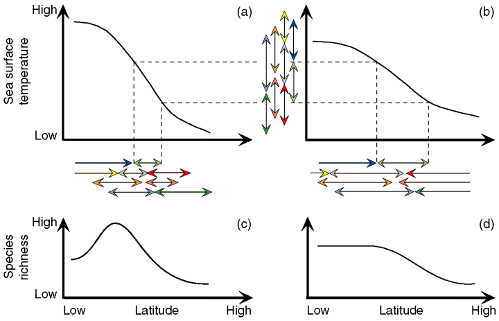
Illustration of the causal effect of the magnitude of the SST gradient on the shape and magnitude of the resulting LGTR. The latitudinal projection (horizontal arrows) of a given random distribution of thermal ranges (vertical arrows) on a steep (a) or weakened (b) SST gradient leads to a steep bimodal (c) or weakened unimodal (d) LGTR, respectively. The different colours of arrows correspond to different species
Our simulations indicate that under present-day Atlantic conditions, simulated clades always generate two peaks of species richness at the latitudes of the Tropics of Cancer and Capricorn while a single modal value should be expected near the equator as a result of the single geographic mid-domain effect. Superimposition of the SST gradient on the simple geographic mid-domain effect splits the expected unimodal LGTR into two roughly symmetric species richness gradients peaking at intermediate latitudes, between maximum and minimum SST values (Fig. 7). This result leads to consider each hemisphere as a bounded thermal domain where the principle of the mid-domain effect effectively applies. The observed bimodal LGTR can thus be interpreted as resulting from the combination of two distinct geometric mid-domain effects: geographic and thermal.
Geographic origin of the first simulated species
In addition to the shape and magnitude of the SST gradient, the geographic location of the first simulated species appears to be important in controlling the location of the LGTR modes. This evolutionary parameter corresponds to an intrinsic phylogenetic control of the biogeographic development of the simulated clade; it by no means implies latitudinally differentiated extinction and/or speciation rates, but simply corresponds to the origination area of the simulated taxonomic group. This effect is very likely to result from the partial inheritance of the thermal range of the mother species during each simulated speciation event. During the simulated history of a clade, some of the new species may thus progressively diffuse away from the thermal range of their common ancestor (Fig. 2).
From this point of view, it appears that a way to obtain a simulated LGTR similar to the one observed for present Atlantic planktonic Foraminifera (and many other taxonomic groups) requires a steep SST gradient and a biogeographic dispersal from middle to low latitudes. This interpretation is consistent with the oversimplified theory that characterizes the tropics as a ‘cradle’ and the poles as a ‘museum’ (Crame 1992, 2001; Chown and Gaston 2000). Conversely, simulations of clades originating at middle to high latitudes always produce LGTR modal values at middle to high latitudes. Although less frequently documented, such high latitudinal modal values are known for Phocidae (Stevens 1989; Proches 2001), some pelagic seabirds (Proches 2001), some bivalves (Crame 2002; Valdovinos et al. 2003), and prosobranchs (Valdovinos et al. 2003).
The latitudinal gradient of Atlantic planktonic Foraminifera
In the case of present-day Atlantic foraminifera, observed and modelled distributions and gradients indicate that species richness clearly decreases with the highest temperatures. This is confirmed by a significant third-order polynomial covariation between species richness and SST values (Rutherford et al. 1999). This bimodal pattern was first interpreted as the consequence of mixed water assemblages near the equatorial convergence between the North and South Atlantic gyres (Rutherford et al. 1999; Clarke and Lidgard 2000). A second hypothesis suggesting that the equatorial SST values are too high to maintain the physiological functioning of foraminifera, has also been proposed by Rutherford et al. (1999). However, as noted by these authors and Bijma et al. (1990), this explanation is not entirely convincing as many foraminifera were bred and reproduced with relatively good success at temperatures higher than the maximum SST values observed in the Atlantic Ocean (c. 30°C).
The similarities observed between the LGTR simulated by our 2D ‘geophyletic’ model and most observed distributions and gradients of species richness (especially for foraminifera (Rutherford et al. 1999; Fig. 5) suggest that, in a given geographic context, a realistic LGTR can be simulated by controlling only two primary drivers: the shape and magnitude of the SST gradient and the geographic origin of the evolutionary history of the clade. The persistence of bimodal gradient in simulations where oceanic currents are suppressed, suggests that the inter-tropical drop of species richness may not result from mixed water assemblages in the convergence zone between the North and South Atlantic gyres. Similarly, the fact that the simulated gradient is unaffected by the values and degree of latitudinal differentiation of speciation and/or extinction rates indicates that no such hypothesis is necessary to generate observed LGTR (fideSax 2001; Hille Ris Lambers et al. 2002; Bromham and Cardillo 2003; contraRohde 1992; Jablonski 1993; Arnold and Parker 1999; Chown and Gaston 2000; Buzas et al. 2002; Crame 2002). Simulated changes in the thermal ranges of species also indicate that the difference of frequency between widespread species having a broad latitudinal range linked to a large (e.g. 15°C) temperature range and restricted species having a narrow latitudinal range linked to a small (e.g. 5°C) temperature range does not eliminate the bimodal structure of the LGTR, but strongly influences its shape by either decreasing or increasing its steepness.
Historical explanation of the drop in present-day equatorial foraminiferal diversity involves the effect of the successive glaciation episodes during Plio-Quaternary times. Such episodes directly controlled the biogeographic distributions of foraminifera and other pelagic organisms by shrinking or expending their geographic ranges (e.g. Lazarus et al. 1995; Wilson 1998; Kandiano et al. 2004). However, alternations between the present-day SST gradient (inter-glacial conditions) and a steeper and colder SST gradient (glacial conditions) during the simulation do not modify the bimodal structure of the LGTR. Therefore, along with other explanations such as differential evolutionary rate or the current effect, this historical hypothesis does not appear to be a fundamental factor in the making of a bimodal LGTR.
Other classically invoked factors not taken into account in our simulations, such as energy availability, productivity, seasonality or geographic area (Rohde 1992), all strongly directly or indirectly covary with latitude. These factors also do not appear necessary for generating a realistic, large-scale bimodal LGTR, although their relative influences remain to be tested with the same type of simulations. This of course does not imply that all of these factors do not participate at local or regional levels (e.g. in generating regions of maximum or minimum richnesses such the Amazon Basin or the Caribbean islands), but it plays down their respective roles as primary causes or limiting factors for the global shape of the large scale LGTR. For instance, the longitudinal discrepancies between the observed and simulated patterns of diversity are certainly because of the effects of these numerous additional factors.
Conclusion
The 2D ‘geophyletic’ model presented in this paper allows realistic simulations of the modern distribution of species richness and bimodal gradient for present Atlantic planktonic Foraminifera. It emphasizes a simple relationship between the observed latitudinal SST gradient and LGTR (Fig. 7). Extending this result to numerous other marine taxonomic groups that also present a bimodal LGTR allows us to hypothesize that a large-scale marine LGTR is a double geometric by-product of the geographic context and of the latitudinal SST gradient combined with the dispersal history of the clade. To a first order, our simulation model suggests that classically invoked biotic or abiotic parameters such as SSC, differential evolutionary rates, ecological associations (Rahbek and Graves 2001; Whittaker et al. 2001) are unnecessary to simulate bimodal large-scale LGTRs. Nevertheless, as all LGTR include local or regional variations and exceptions, such second order parameters are obviously required to explain the finer structure of the pattern of taxonomic richness. In this context, it seems logically difficult to consider only one biotic (e.g. physiologic) or abiotic (physical environment) parameter as the single deterministic cause in the development of marine LGTRs. Thus, other proposed factors underlying a LGTR should be tested with similar models to see if similar patterns emerge. Moreover, similar models should ideally be constructed with different clades to test if thermal range, dispersion ability, diversity threshold or other parameters help to modulate the formation and evolution of bimodal diversity pattern. To complement this, a third dimension (e.g. depth of marine species) should be added: in the special case of Foraminifera, the role of depth (also related to the thermal gradient) has been identified in speciation processes (e.g. Schneider and Kennett 1999). Subsequently, a 3D model, while computationally much more time-consuming, could greatly improve and refine the resulting simulated diversity pattern.
In the absence of other constraints, the results of null models based on the mid-domain effect may not always yield realistic results (e.g. Koleff and Gaston 2001; Hawkins and Diniz-Filho 2002; Valle de Britto Rangel and Diniz-Filho 2003; Zapata et al. 2003). However, when used in combination with climatic and evolutionary constraints, this type of probabilistic model can reproduce the essential patterns of LGTR. In turn, the better characterization of the non-linear relation between a given SST gradient, and the corresponding global structure of a large scale LGTR, enables prediction of the relative changes in the shape, magnitude and evolution of past SST gradients for well-documented fossil LGTRs (Brayard et al. 2004).
Acknowledgements
We thank S. Legendre (UMR-CNRS 5125, Lyon) and P. Linder (University of Zürich) for stimulating comments on an earlier draft version and two anonymous reviewers for insightful remarks on a first version of this paper. Three JZSER reviewers, F. Cecca, R.K. Colwell and N. MacLeod, provided constructive critics which helped us to improve the manuscript. M. Williams (British Antarctic Survey) and S. Gilder (Institut de Physique du Globe, Paris) kindly improved the English spelling. This work was supported by the Swiss NSF project 2100-068061.02 (A.B. and H.B.), the program CNRS/INSU-Eclipse, project 00-10 (A.B. and G.E.), and a Rhône-Alpes-Eurodoc grant (A.B.).


