Disregarding the edaphic dimension in species distribution models leads to the omission of crucial spatial information under climate change: the case of Quercus pubescens in France
Abstract
Species distribution modelling is an easy, persuasive and useful tool for anticipating species distribution shifts under global change. Numerous studies have used only climate variables to predict future potential species range shifts and have omitted environmental factors important for determining species distribution. Here, we assessed the importance of the edaphic dimension in the niche-space definition of Quercus pubescens and in future spatial projections under global change over the metropolitan French forest territory. We fitted two species distribution models (SDM) based on presence/absence data (111 013 plots), one calibrated from climate variables only (mean temperature of January and climatic water balance of July) and the other one from both climate and edaphic (soil pH inferred from plants) variables. Future predictions were conducted under two climate scenarios (PCM B2 and HadCM3 A2) and based on 100 simulations using a cellular automaton that accounted for seed dispersal distance, landscape barriers preventing migration and unsuitable land cover. Adding the edaphic dimension to the climate-only SDM substantially improved the niche-space definition of Q. pubescens, highlighting an increase in species tolerance in confronting climate constraints as the soil pH increased. Future predictions over the 21st century showed that disregarding the edaphic dimension in SDM led to an overestimation of the potential distribution area, an underestimation of the spatial fragmentation of this area, and prevented the identification of local refugia, leading to an underestimation of the northward shift capacity of Q. pubescens and its persistence in its current distribution area. Spatial discrepancies between climate-only and climate-plus-edaphic models are strengthened when seed dispersal and forest fragmentation are accounted for in predicting a future species distribution area. These discrepancies highlight some imprecision in spatial predictions of potential distribution area of species under climate change scenarios and possibly wrong conclusions for conservation and management perspectives when climate-only models are used.
Introduction
The impact of climate warming on species distribution is now well established worldwide, depicting primarily poleward and upward range shifts (e.g. Parmesan, 2006; Lenoir et al., 2008; Bertrand et al., 2011b). In this context, conservation and management concerns about natural ecosystems have arisen (e.g. Lindenmayer et al., 2008; Richardson & Whittaker, 2010), and the modelling approach based on species distribution models (SDMs) has been widely used since the 1990s to predict the future potential species distribution area from climate scenarios (e.g. Guisan & Thuiller, 2005; Araujo et al., 2011; Engler et al., 2011; Thuiller et al., 2011). However, as Austin and Van Niel (2011a,b) have recently underscored, the use of SDMs needs to be revisited with respect to the ecological framework, particularly in relation to climate change scenarios. In particular, they recommended ensuring that predictors selected in SDM describe an ecophysiological process in the species' development and include both climatic and non-climatic variables at a spatial resolution compatible with the ecological process.
The spatial distributions of species are often studied with regard to climatic variables alone (climate-only or bioclimatic model; e.g. Huntley et al., 1995; Sykes et al., 1996; Araujo et al., 2011; Engler et al., 2011; Thuiller et al., 2011). This practice assumes that climate conditions alone are sufficient for predicting the primary changes in species distribution under climate scenarios at a large extent (national or continental extent) and often at coarse spatial resolution (10 × 10–50 × 50 km; Pearson & Dawson, 2003). The validity of climate-only models has been questioned on the grounds that many factors other than climate can significantly influence species distributions and distribution changes (e.g. Coudun et al., 2006; Marage et al., 2008; Meier et al., 2010; Keenan et al., 2011) and must be applied only with a thorough understanding of their limitations (e.g. Hampe, 2004; Heikkinen et al., 2006). Austin and Van Niel (2011a,b) denounced this current practice by demonstrating that omitting non-climatic variables (light and topography in their example; edaphic dimension based on expert opinions was insignificant) in SDM to predict the future potential distribution of Eucalyptus fastigata across the 21st century underestimates the area of its optimal habitat and prevents the definition of crucial refugia for its persistence and colonization. Edaphic variables, which depict nutrient availability and soil toxicity for plants and depend on the local heterogeneity of the soil, are expected to increase the accuracy of future predictions and to confound outputs derived from climate-only models (Lafleur et al., 2010; Austin and Van Niel, 2011b). Edaphic factors have been shown to determine a significant part of plant growth (e.g. Bontemps et al., 2011) and distribution (e.g. Coudun et al., 2006; Bertrand et al., 2011a). However, the nutritional dimension is scarcely included in SDMs because of the lack of available and accurate grids over large extents (Dengler et al., 2011).
In this study, we investigated the contribution of edaphic factors in bioclimatic SDMs to predict robust and accurate potential species distributions under climate change scenarios on a broad extent (~546 000 km²). We compared the niche spaces of Quercus pubescens derived from climate-only and climate-plus-edaphic models, as well as spatial predictions computed from them across metropolitan France and over the 21st century using two climate change models and scenarios (PCM B2 and HadCM3 A2). Our future predictions performed here are based on dynamic and stochastic simulations combining SDM and a cellular automaton accounting for seed dispersal distance, forest fragmentation and life history traits for Q. pubescens (Franklin, 2010). Following the results of Austin and Van Niel (2011b) and Lafleur et al. (2010), we hypothesized that edaphic variables are essential predictors for predicting the potential distribution changes under climate change at a large scale. We addressed two specific questions through the example of Quercus pubescens: (1) How different are the niche spaces derived from climate-only and climate-plus-edaphic models? (2) What are the spatial consequences of accounting for the edaphic dimension to the future distributions predicted under climate change scenarios?
Material and methods
Ecology of Quercus pubescens
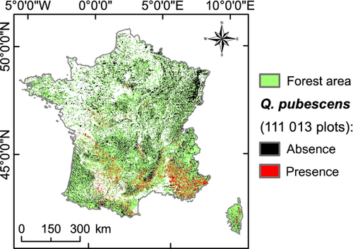
Q. pubescens is a long-lived submediterranean tree species that occurs mainly in the South of Europe and that is distributed in France over the Southern half of the country (Rameau et al., 2008; Fig. 1). It is a heliophilic, thermophilic species requiring a low-to-medium soil water capacity. Q. pubescens primarily occurs on calcareous soils, but tolerates acidophilous conditions. The resistance of this species to cold events on calcareous soils explains its presence in the Northern half of France and its occurrence at elevations up to 1400 m (Rameau et al., 2008).
Specific information about the life cycle of this species is scarce. The age of first reproduction for various Quercus species ranges from 3 growing seasons old for the short-lived Quercus species to 30–45 years for the long-lived Q. petraea (reaching up to 1000 years old; Ducousso et al., 1993). Acorn production varies highly between years (Ducousso et al., 1993). In Europe, acorns of Quercus species are mainly dispersed by rodents and the European jay (Garrulus glandarius; Den Ouden et al., 2005). Jays cache acorns over a greater distance than rodents, leading to 2 peaks in distance distribution: one close to the parent trees and another several hundred metres away from them (Schuster, 1950; Den Ouden et al., 2005). Dispersal distance can reach 7 km (Schuster, 1950). Even if these long-distance dispersal events are rare, they are crucial to explaining the spread of Quercus species since the last glacial period (Le Corre et al., 1997).
Species dataset
Presence/absence data for Q. pubescens, including the year and location of the plots, were compiled from 3 French databases (EcoPlant, Sophy, and NFI). EcoPlant (Gégout et al., 2005) is a phytoecological database integrating approximately 145 different study sources between 1905 and 2007; 5367 forest plots were used from this database. Sophy (Brisse et al., 1995) is a phytosociological database that includes more than 4600 different study sources (in forests and open landscapes) from the last century; 31 307 forest plots were used from this database. For the EcoPlant and Sophy databases, the floristic plots within forest habitats were performed across a surface area of about 400 m². NFI is the database of the French National Forest Inventory (Robert et al., 2010). From 1987 to 2004, the NFI sampling method was based on a systematic grid (1 km²) of plots in each administrative unit and was repeated every 12 years (Robert et al., 2010). In 2004, the sampling design was changed to cover the entire French forest areas on a yearly basis. The system is now based on a systematic national grid of 10 km², which is moved 2 km each year, thereby ensuring a 1-km2 coverage of forest habitats every 10 years (Robert et al., 2010). For the NFI database, all floristic plots were performed across a surface area of about 700 m²; 130 819 forest plots were used from the NFI database.
To minimize both the over sampling of some geographical regions and environmental conditions and the effect of spatial autocorrelation that can bias SDMs, we conserved only the sites separated by more than 1 km. Thus, we fitted both the climate-only and climate-plus-edaphic SDMs of Q. pubescens from 111 013 forest plots encompassing 19 624 species occurrences between 1961 and 2008 (Fig. 1).
Environmental variables included in the SDMs
The environmental variables were selected to cover the primary factors for plant species distribution (energy, water, light and nutritional resources; Austin & Van Niel, 2011b). Environmental variables described below focus on the factors the most relevant to explain the distribution of Q. pubescens (see Supplementary Methods for more details about the pool of environmental variables tested). We used the mean temperature of January (Tm1) as a proxy of energy limits. The available water was represented by the climatic water balance of July (CWB7; precipitations–potential evapotranspiration, based on the work of Turc 1961). Mean temperature and precipitations grids for 1961–1990 were provided by the meteorological model AURELHY spatialized at a 1-km2 resolution (Bénichou & Le Breton, 1987). Light and topography variables were not directly included in the SDMs because both variables are already accounted for by climatic water balance (partially determined by solar radiation), precipitations and temperature variables (based on elevation and embankment topography; see Supplementary Methods for more details). The collinearity between Tm1 and CWB7 was low over the calibration dataset (R² = 0.42).
The edaphic dimension included in the climate-plus-edaphic SDM was characterized by soil pH, which represents a complex gradient that has a direct physiological effect on plant growth. In particular, soil pH describes a decreasing gradient of Al toxicity for plants (Cronan & Grigal, 1995). Soil pH was also used to account for soil nutritional status as it controls the uptake of minerals by plants and is correlated with many edaphic factors (Schoenholtz et al., 2000). Soil pH was provided by the 1-km² French soil pH grid (http://www.ifn.fr/spip/spip.php?rubrique182&rub=cat). The soil pH grid was achieved by (i) inferring optimum pH requirements for 511 plant species (Gégout et al., 2003) derived from 3835 EcoPlant plots coupling species occurrences and the pH values of the upper organo-mineral A horizon of soils (pH H20 laboratory measured) and (ii) the interpolation of bio-indicated pH values computed as the mean of the optimum pH requirements of at least five plants occurring on each plot of 104 375 NFI plots (inventoried between 1989 and 2004; Gégout et al., 2003). This grid provides a good estimation of pH values throughout the French forest territory (R² between measured and bio-indicated pH values = 0.58; SD of predictions = 0.81; n = 261 independent plots regularly distributed over France) and does not affect SDM outputs compared with measured pH values (see Supplementary Methods). The collinearity between soil pH and climatic variables were very low over the data set used to fit the SDMs (R² with Tm1 = 0.005; R² with CWB7 = 0.199). In the absence of future projections of soil pH under global change, pH was considered constant to predict the future potential distribution area of Q. pubescens.
Future climatic projections
Future projections of the mean temperature of January and the climatic water balance of July were used to derive the potential distribution of Q. pubescens over the 21st century from the climate-only and climate-plus-edaphic models. Two extreme climate projections were used to browse the range of climate conditions expected over the 21st century. First, we used the B2 scenario of the PCM model (Washington et al., 2000), in which atmospheric CO2 rises from 380 ppm in 2000 to 800 ppm in 2100. The mean temperature of January and the climatic water balance of July, which were equal to 3.1 °C and −72.5 mm for 1961–1990, are predicted to reach 5.4 °C and −88.5 mm, respectively, for 2091–2100 throughout the French territory. Second, we used the A2 scenario of the HadCM3 model (Johns et al., 2003), in which atmospheric CO2 reaches 1250 ppm in 2100. The mean temperature of January and the climatic water balance of July are predicted to reach 7.7 °C and −124.1 mm, respectively, for 2091–2100 throughout the French territory. Monthly mean temperature, precipitation and nebulosity grids were provided by the Tyndall Centre for Climate Change Research at a spatial resolution of 10′ × 10′ (i.e. ~15-km² at the French scale) and at a decadal time scale between 2001 and 2100 (Mitchell et al., 2004). We downscaled the climatic projections to a 1-km² resolution by adding the anomaly between future predictions and mean climate conditions over 1961–1990 to the referential climatic grids used to fit SDMs.
Fitting SDMs
Generalized additive models (GAM; Hastie & Tibshirani, 1990) with binomial likelihoods were used to model the environmental dependence of the presence/absence of Q. pubescens. GAM is a simple statistical method commonly used by species distribution modellers to avoid arbitrary mathematical formulations of the response curves (Yee & Mitchell, 1991). We fitted the climate-only and climate-plus-edaphic SDMs through the equations f(PQpub) = s1(Tm1) + s2(CWB7) and g(PQpub) = s3(Tm1) + s4(CWB7) + s5(pH), respec-tively, where f and g are the logistic link function, PQpub is the probability of presence of Q. pubescens conditional to the environmental state, and sx are smoothing functions for environmental indicators, estimated non-parametrically with local cubic splines. We limited the degrees of freedom of the smoothness to four. See Supplementary Methods and Table S1 for more details about the process and results of the environmental variable selection.
We assessed the effect of edaphic and climatic variables in the SDMs by an analysis of deviance (Hastie & Tibshirani, 1990). As recommended by Liu et al. (2011), we evaluated the performance of the models from both the goodness-of-fit of the models and the discriminatory power of the models. We computed the D² value as a proxy of goodness-of-fit of each model: D² = 100 × (null deviance – model deviance)/null deviance. The deviance is a generalization of the residual sum of squares in ordinary regression and is derived from the likelihood functions (L) (model deviance = −2 × ln(L); Hastie & Tibshirani, 1990). D² represents the percentage of deviance explained by environmental variables included in the model (analogous to R² in regression; Yee & Mitchell, 1991). We also computed the area under the curve (AUC) of the receiver operating characteristics curve, the global success (S, correct classification rate of both presence and absence), sensitivity (Sn, correct classification rate of presence) and specificity (Sp, correct classification rate of absence) as proxies of the discriminatory power of each model (Liu et al., 2011). As the SDMs were fitted from the same geographical extent and data set, these proxies could be used to compare the predictive performance between them (Lobo et al., 2008). All these statistics were computed by random replications (n = 3000 replications). In each replication, SDMs were fitted using a random 10% of the 111 013 forest plots, and D², AUC, S, Sp, Sn were computed from 10% of the remaining forest plots in order to minimize the potential spatial dependence between calibration and validation datasets. Moran's I was also computed from residuals of each SDM to assess the effect of spatial autocorrelation in the calibration of models (I varies between −1 and 1; absence of autocorrelation is closed to 0) (Fortin & Dale, 2005; Dormann et al., 2007). The effect of spatial resolution on the significance of the variables included in SDM was tested by adjustment of models from 1 × 1, 10 × 10, 25 × 25 and 50 × 50 km grids of both environmental factors and presence/absence of Q. pubescens (see Supplementary Methods). SDMs and statistics were computed in the R environment (R Development Core Team, 2010).
Dynamic future predictions using a cellular automaton
We implemented a cellular automaton in the R environment (R Development Core Team, 2010), named simRShift, to account for the seed dispersal distance of Q. pubescens over the French forest areas in future predictions of its distribution under global change. Current and future spatial projections of climate-only and climate-plus-edaphic SDMs were performed each decade between 2010 and 2100 for both climate change scenarios at a 1-km² resolution. These grids represent the habitat suitability of Q. pubescens under global change. Assuming no substantial change in land-use over the 21st century, we restricted projections to open and closed forest areas derived from Corine Land Cover 2006, the only ecosystems where this species occurred naturally. The initial distribution of this oak species was defined from observed data exhibiting a meta-population covering 19 624 km² (Fig. 1). As Q. pubescens is a long-lived species, we distinguished two life stages: juvenile (non-reproductive life stage) and mature (reproductive life stage). We fixed the age of first reproduction to 20 years old. We assumed that the initial meta-population was composed only of mature individuals, because of the lack of age information in the observed data. The initial juvenile meta-population was achieved by simulating establishment events over 19 years under the referential environmental conditions used to fit the SDMs. Future simulations of the potential distribution of Q. pubescens start in 2011 from this state.
Two main demographic processes driven by environmental changes were included in simRShift: survivorship/mortality and colonization (Engler & Guisan, 2009; Franklin, 2010). Without an explicit survivorship/mortality model for Q. pubescens, we assumed that environmental conditions favouring its presence were also favourable to its survivorship. Thus, in the first year of each decade (representing changes in environmental conditions due to climate change), the survivorship/mortality of Q. pubescens in each pixel this species occupied at the end of the previous decade was computed as a sampling extraction of this binary event conditional to the probability of presence extracted from the habitat suitability grid at the time experienced. This approach is an alternative method to the commonly used ‘probability threshold’ to pass from the probabilities of presence (i.e. a continuous variable) to a binary variable (e.g. presence/absence, survivorship/mortality, dispersion/no-dispersion; e.g. Engler & Guisan, 2009; Early & Sax, 2011; Engler et al., 2011; Meier et al., 2012). In particular, the selection of a ‘probability threshold’ can be non-optimal and for instance, may lead to predicting the absence of a species when the species is in actuality present (Liu et al., 2005). The sampling extraction used allows this bias to be avoided, which can be important as false predictions of absence can readily occur at the margins of a species distribution area.

Finally, because predictions in simRShift included some randomness, we performed 100 simulations. Simulations were conducted yearly using both the climate-only and climate-plus-edaphic SDMs under the PCM B2 and HadCM3 A2 climate scenarios. Spatial predictions of the potential distributions were summed at the end of each decade (i.e. 2010, 2020… 2100) to report the occurrence of Q. pubescens. Changes in parameters, such as seed dispersal distance and age of first reproduction, had low impact on the results (Figs S2 and S3). Thereafter, results concerned only the evolution of the mature meta-population under global change.
Results
Current projections of SDM
Climate-only (SDMc) and climate-plus-edaphic (SDMce) models were highly significant (comparison with null model by analysis of deviance: P < 2.2.10−16). Adding soil pH to the climate variables substantially improved the goodness of fit of the SDM (mean D² of SDMc and SDMce [SD] = 35.48% [0.87] and 48% [0.92] respectively; comparison of models by analysis of deviance: P < 2.2.10−16). We also found that the discriminatory power of the SDMce (mean AUC [SD] = 0.929 [0.004]) was better than that of the SDMc for Q. pubescens (mean AUC [SD] = 0.887 [0.005]). We observed that accounting for the nutritional dimension increased the global success of prediction of the SDM (mean S [SD]= 82.16% [1.1] in SDMc and 86.72% [0.89] in SDMce), both for the presence (mean Sn [SD] = 82.51% [1.72] in SDMc and 85.91% [1.36] in SDMce) and the absence (mean Sp [SD] = 82.08% [1.62] in SDMc and 86.89% [1.27] in SDMce) of Q. pubescens. We observed lower spatial autocorrelation in SDMce than in SDMc (Moran's I = 0.088 and 0.246 in residuals of adjacent pixels [<1.5 km] respectively; Fig. S4). CWB7, Tm1 and pH were significant whatever the spatial resolution used (1 × 1–50 × 50 km), and the weight of soil pH in SDM increased at coarser resolutions (Table S3).
We found strong differences in the ecological niches derived from the SDMc and SDMce (Fig. 2). In particular, we showed an important shift in the optimal climate conditions towards lowest water deficit of July (+17 mm in CWB7) and hottest temperature of January (+3.6 °C in Tm1) when soil pH was considered in the SDMs (Fig. 2). We also found an increase in the climate tolerance of Q. pubescens in the SDMce when the pH increased (pH > 6; Fig. 2). The SDMce predicted a higher probability of presence of Q. pubescens primarily (i) when low water deficit of July occurred, and (ii) when both hot climate of January and dry climate of July occurred (Fig. 2). When the soil pH was less favourable to Q. pubescens (i.e. on acid soils), it occurred only for specific climate conditions close to the optima ones.
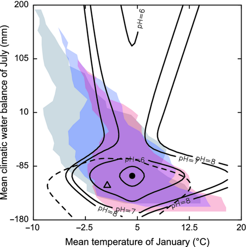
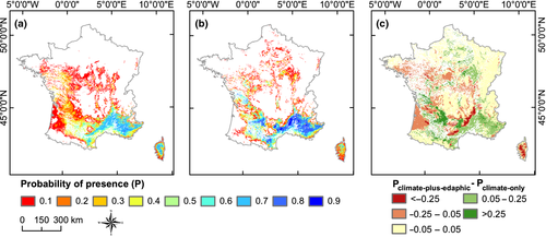
These discrepancies in the niche-space definition of Q. pubescens highly structured the current spatial projection of its potential distribution area (Figs 2 and 3). We observed that the potential habitat for Q. pubescens (delimited by a probability of presence >0.1) derived from the SDMce covered a smaller forest area and showed a higher level of probability of presence in average compared to the SDMc (−26 266 km², which corresponds to 16.2% of the climatic envelope and +0.09 in probability; Fig. 3). The spatial projection of the SDMce exhibited 19 532 km² of potential habitat that was not predicted by the SDMc. We observed the emergence of patches potentially suitable for Q. pubescens on basic soils, especially in the North of France where the lowest water deficit of July occurs (14 090 km²; Fig. 3). In the South of France where the hottest temperature of January and the driest climate of July occur, we found higher probabilities of presence predicted from the SDMce than from the SDMc (+0.11 in probability [SD = 0.16]; Fig. 3). We also reported that the current potential distribution area of Q. pubescens predicted from the SDMce was more fragmented than the one predicted from the SDMc (Fig. 3).
Simulations of future projections
The simulations of the future potential distribution area of Q. pubescens based on the SDMc and SDMce differed substantially over the French forest territory in 2100, regardless of the climate scenario used (Fig. 4). For 2100, we showed that 55.1% and 38.2% of the potential habitat areas occupied by Q. pubescens (delimited by a species occurrence >10 out of the 100 simulations) were shared in common between simulations based on both SDMs under the PCM B2 and HadCM3 A2 climate scenarios respectively. In comparison, 66.7% and 47.8% of the potential habitat areas (delimited by a probability of presence >0.1), as directly projected from both SDMs (i.e. without accounting for dynamic processes such as seed dispersal and the spatial fragmentation of the forests), were shared between these SDMs under the PCM B2 and HadCM3 A2 climate scenarios respectively.
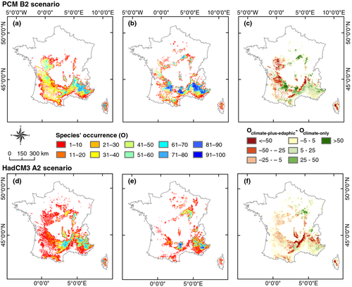
From the 100 dynamic simulations, we observed that the mean level of species' occurrence predicted from the SDMce was lower at the French scale than that predicted from the SDMc when the greatest climate warming occurred (−6 occurrences out of 100 simulations on average under HadCM3 A2). However, we report that the highest species' occurrences were predicted by the SDMce in both the Northern boundary of the distribution area and the Mediterranean region (except in Corsica). Both of these areas depicted numerous refugia and favourable areas for the development of Q. pubescens in confronting climate change where optimal soil conditions occurred.
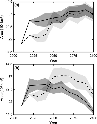
We predicted that the mean potential area occupied by Q. pubescens greatly increased for the first decade in the simulations based on the SDMce relative to those based on the SDMc (Fig. 5). While we observed a continuous increase leading to the convergence of the mean surface area simulated from both SDMs under the PCM B2 scenario from 2050 (mean difference [SD]= 485 km² [5084] in 2100, Paired Student t test: P = 0.34; Fig. 5a), the HadCM3 A2 climate scenario leads to a largest mean surface simulated from the SDMc (mean difference [SD] = 9796 km² [3181] in 2100, Paired Student t test: P < 2.2.10−16; Fig. 5b). Under this hottest climate scenario, the mean potential areas decreased after 2040 and 2070 in simulations based on the SDMce and SDMc respectively. Predictions of the mean surface potentially occupied by Q. pubescens were the greatest under the PCM B2 climate scenario, regardless of the SDM used in the simulations (Figs 4 and 5).
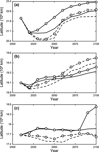
We also predicted a northward shift in the potential distribution area of Q. pubescens over the 21st century, irrespective of the SDMs and climate scenarios considered in the simulations (compared Figs 1, 4, and 6). We observed that accounting for the nutritional dimension in the future simulations led to the greatest northward shift of the Southern (+21 and +91 km in 2100 under the PCM B2 and HadCM3 A2 climate scenarios respectively) and Northern (+44 and +57 km) boundaries of the distribution area (Fig. 6a, c). These shifts were especially marked for the HadCM3 A2 scenario. In contrast, the northward shift of the median latitude was higher when we simulated the future distribution considering climate variables alone (+15 and +16 km in 2100 under the PCM B2 and HadCM3 A2 climate scenarios respectively; Fig. 6b). We also found an upward shift in the median altitude and in the top and bottom boundaries of the distribution area under the HadCM3 A2 climate scenario (Fig. S5). Accounting for the nutritional dimension in the simulations led only to a greater upward shift of the bottom boundary (+22 and +58 m under the PCM B2 and HadCM3 A2 climate scenarios respectively); otherwise, the shifts were comparable between the SDMs (Fig. S5).
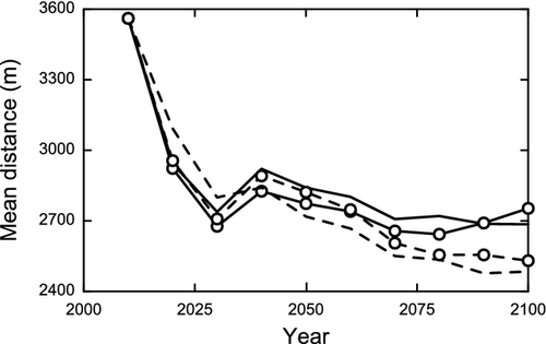
We predicted that the distribution area of Q. pubescens accounting for the nutritional dimension was composed of a greater number of patches (+2036 and +268 patches in 2100 under PCM B2 and HadCM3 A2 respectively; Fig. 7) with a lower mean surface area (−869 and −823 m²) and a greater distance between patches (+223 and +201 m in average) than simulations based on climate variables alone (Fig. S6). This apparent spatial fragmentation of the distribution area is higher under the HadCM3 A2 climate scenario (Figs 4 and 7).
Discussion
Adding new relevant variables to a bioclimatic envelope and the use of a dynamic approach to simulate species migrations have been recently highlighted as important ways to improve the accuracy of predicting the future species distribution under global change (Franklin, 2010; Lafleur et al., 2010; Austin & Van Niel, 2011a,b). Here, we demonstrated the divergent outputs achieved when climate variables were considered alone or in conjunction with a nutritional variable for Quercus pubescens across metropolitan France (~546 000 km²). Future predictions were computed from a more dynamic approach than that derived directly from SDMs. They were based on the combination of a SDM and a cellular automaton (simRShift), a more mechanistic approach accounting for the spatial fragmentation of forest habitat, seed dispersal limitations and life history traits, as determined from the autecology and life cycle of Quercus species (e.g. Ducousso et al., 1993; Den Ouden et al., 2005; Rameau et al., 2008). All these factors are important for assessing accurately the potential range shifts in a species distribution (Franklin, 2010). In contrast to similar studies using such a dynamic approach (e.g. Engler & Guisan, 2009; Early & Sax, 2011; Engler et al., 2011; Meier et al., 2012), simRShift used an original method to compute survivorship, reproduction and colonization within a pixel. The use of a ‘probability threshold’ can be non-optimal for passing from a continuous variable (e.g. the probability of presence) to a binary variable (e.g. presence/absence) and often leads to inaccurate predictions (Liu et al., 2005). Here, all the ecological events were computed as a sampling extraction of a binary event (e.g. the survivorship or death of a species) conditional on the probability of presence extracted from the habitat suitability grid (i.e. spatial projection of SDM). As a consequence, our future predictions can be improved by including explicit survivorship and reproduction models for Q. pubescens in our approach, as well as by differentiating the SDMs of juvenile and mature stages (Bertrand et al., 2011a; Urbieta et al., 2011). However, these potential improvements should not change our present conclusions because only the consideration of the edaphic dimension changes in our future predictions. The initial distribution of Q. pubescens that we used is based on field observations rather than on spatial projections of SDMs in order to not bias spatial comparisons over the 21st century with different and overestimated initial distributions predicted from climate-only and climate-plus-edaphic SDMs. As a consequence, this choice leads to a sharp increase in the surface area occupied by Q. pubescens the first years in the simulations (i.e. transition from field observations to predictions), but it does not challenge our results because the initial distribution is the same in each simulations.
Despite the numerous studies highlighting some of the limitations in using bioclimatic models to predict the potential distribution area of a species (e.g. Hampe, 2004; Heikkinen et al., 2006), these models are still used (e.g. Araujo et al., 2011; Engler et al., 2011; Thuiller et al., 2011). Studies that consider that climate conditions alone are the main large-scale drivers of species range shifts during climate change (Pearson & Dawson, 2003), view other factors, such as nutrient (Coudun et al., 2006; Bertrand et al., 2011a) or light (Austin & Van Niel, 2011a,5) availability, as important for the niche-space definition, but as acting at a more local scale, and as providing only a small contribution in predicting future species distributions. Contrary to these assumptions, we highlighted that soil pH contributed significantly to the niche-space definition of Q. pubescens until at least 50 × 50 km spatial resolution, and its weight increased at coarser resolutions. As Coudun et al. (2006) had already shown for Acer campestre, we also reported that climate-plus-edaphic model better characterized niche space of Q. pubescens, which is more consistent with its autecology (Rameau et al., 2008). Disregarding the edaphic dimension leads to omitting the combination effect of climate and edaphic variables, which affect the definition of the optimal condition for Q. pubescens and its tolerance in facing climate change. As a consequence, these differences lead to important discrepancies when the current habitat suitability of Q. pubescens and the predictions of its potential distribution range shifts under climate scenarios are mapped. Considering the nutritional dimension improved the spatial accuracy of the predictions excluding unsustainable soil conditions for Q. pubescens in the bioclimatic envelope (i.e. acidic soil). The spatial projections based on climate variables alone may overestimate both the surface and the contiguity of the potential habitat of Q. pubescens, leading to low spatial concordance between the climate-only and climate-plus-edaphic simulations. The extrapolation of the climate-plus-edpahic SDM under novel climate conditions may lead to overestimate the probability of presence, especially where high value of climatic water balance of July is predicted (Fig. 2). However, this specific case is limited in area to only 1144 and 140 km² under PCM B2 and hadCM3 A2 climate change scenario in 2091–2100, respectively, and therefore it does not bias our future predictions. The greatest tolerance for climatic constraints, as defined by climate-plus-edaphic SDM, increased the level of probability of presence (or species' occurrence in the case of future predictions) under favourable soil conditions (i.e. basic soils). This resulted in the emergence of sustainable patches for Q. pubescens in the Northern part of its distribution, consistent with current field observations and also in the Southern part of its distribution area (mainly over the Mediterranean region). These patches were crucial local refugia that contributed greatly to the northward range shift and the expansion of the potential distribution area, and to the local persistence of Q. pubescens under climate change over the French forest territory.
Refugia have played a great role in the past for the persistence, migration and evolution of species (e.g. Petit et al., 2003; Linares, 2011). Refugia are expected to fill the same functions under the current and future global change, and identifying their location has become a crucial issue for conservation (Ashcroft, 2010). SDM is a useful tool to define refugia under global change, but the spatial accuracy of the outputs (which differentiate microrefugia to macrorefugia) is often linked to the spatial resolution of the environmental grids used (Ashcroft, 2010). So far, topography or landscape physiography, geographical position, lithology and climate conditions have been identified as the main factors defining refugia under global change (Ashcroft et al., 2009; Dobrowski et al., 2009; Austin & Van Niel, 2011b; Dobrowski, 2011; Ohlemüller et al., 2012; Keppel et al., in press). Here, we showed that the nutritional resource is also an important factor to define local refugia considering its spatial heterogeneity and its importance for plant development (Coudun et al., 2006; Bertrand et al., 2011a; Bontemps et al., 2011). Added to climate variables, it predicted accurate boundaries of the distribution area of Q. pubescens and it also predicted accurate estimations of its probability of presence within this area, highlighting novel refugia and corridors. These ‘climate-plus-edaphic’ refugia and corridors were especially important when seed dispersal and spatial fragmentation are considered, by increasing spatial discrepancies between future distributions areas predicted with and without edaphic dimension.
The spatial discrepancies between predictions based on climate-only and climate-plus edaphic models are especially strong compared with those from the effect of light and topography on the bioclimatic envelope (Luoto & Heikkinen, 2008; Austin & Van Niel, 2011a). These differences are probably explained by a lower correlation between edaphic and climate variables than between light (or topography) and climate variables over the landscape. Soil pH has allowed decreasing drastically the spatial autocorrelation in SDM proving that climate variables are not sufficient to predict an accurate and unbiased spatial distribution of Q. pubescens. All these observations strengthened the importance of having available grids of edaphic variables for predicting the potential range shifts in species distributions. However, such variables are scarce, which often explains why they are not considered (Dengler et al., 2011). Although often decried, indicator values are a useful substitute for inferring environmental variables from plant assemblages in the absence of available measurements (see Diekmann, 2003 for a review, Wamelink et al., 2005), especially when a powerful method is applied to a large georeferenced floristic database (see Bertrand et al., 2011b for an application on the temperature gradient).
In a context where current species range shifts in response to climate warming have been highlighted (Parmesan, 2006; Lenoir et al., 2008; Bertrand et al., 2011b), species distribution modelling is an easy, persuasive and useful tool for anticipating species distribution shifts (Guisan & Thuiller, 2005; Araujo et al., 2011). In the present study, considering the edaphic dimension in the SDMs led to highly divergent outputs for the species' conservation and management plan. Thus, when we considered only the bioclimatic envelope, the potential habitat of Q. pubescens over the 21st century covered a large and contiguous area. In this case, Q. pubescens is considered a species with a high potential persistence in facing climate change and with only small potential range shifts compared with its current distribution. This overall pattern was maintained even under a warmer climate change scenario and in consideration of seed dispersal limitation, forest fragmentation and a later age of reproduction. In contrast, simulations based on climate-plus-edaphic model predicted more reduced and fragmented potential habitats as the climate warmed, so that some corridors and potential area for the species were filtered out. However, the simulations also highlighted some crucial refugia for improving the persistence of the species in its current range and in facilitating its migration in novel favourable environmental conditions in response to climate change. The precision reached by the edaphic dimension provides important decision support for managers. It allows accurate inferences in terms of potential range shifts, the identification of potential corridors of migration for the species and areas where management acts could be engaged (or not) to help species, in particular by not expending resources in areas unsustainable for the species. Although our analyses focused on a unique species, such conclusions may be extended to numerous plants by considering the importance of the edaphic dimension in the niche-space definition of plant species and for species migration (Coudun et al., 2006; Lafleur et al., 2010; Bertrand et al., 2011a), and the importance of seed dispersal and spatial fragmentation in dealing with climate change through migration (Franklin, 2010; Bertrand et al., 2011b). A similar study should be conducted on numerous species to confirm the global importance of edaphic dimension to monitor and to predict plant range shifts under climate warming.
Acknowledgements
We thank G. Riofrío-Dillon, P. Mérian, J-D. Bontemps and J. Lenoir for their helpful comments. We also thank I. Seynave for the management of the EcoPlant database; H. Brisse, P. de Ruffray, C. Vidal, J. Drapier and F. Morneau for their contributions to the Sophy and NFI databases; all who have participated in the conception of the EcoPlant, Sophy and NFI databases. EcoPlant database was funded AgroParisTech, the National Forest Department (ONF) and the French Agency for Environment and Energy Management (ADEME). This study was funded through a PhD grant to R.B. by ADEME and the Regional Council of Lorraine.


