Phylogenetic signal in morphometric data

Sir,

Count us as fans of the new landmark optimization methods recently developed by Catalano et al. (2010) and Goloboff and Catalano (2010). These build on the retooling of TNT to handle continuous data (Goloboff et al., 2006, 2008), which we enthusiastically employed to give us phylogenetic hypotheses for species currently beyond the reach of molecular systematics and lacking many codable characters (Clouse et al., 2009; de Bivort et al., 2010). We are explicit on this point, lest our comments herein about partial warps be construed as a call to return to that method of using morphometrics in phylogenetics. Partial warps are nearly taboo, having stumbled in a notorious simulation (Naylor, 1996) and being rejected as incapable of working by one of their original advocates (Zelditch et al., 2004). They are two-dimensional translations of three-dimensional, landmark-localized, minimal bending energy (principal warps), transformed to eliminate geometrically uniform (affine) scaling and rotations across the whole shape (Bookstein, 1991; Zelditch and Fink, 1995)—a calculation sufficiently complex to repel those who cringe at pre-analysis backflips in phylogenetic data, and sufficiently removed from any known biological process to provide ample fodder for criticism when failing to find the true tree. A reanalysis of the cartoon fish by MacLeod (2002) using relative warps (akin to a principal component analysis of principal warps, which are partial warps minus the two-dimensional translation) did find Naylor’s simulated relationship as the single most parsimonious tree, but it was also complex and perhaps thus not the subject of much further discussion: landmarks were grouped into localized regions, registered across all taxa, relative warps were calculated for each group, and then taxa were clustered by the two most important relative warps in each group to generate codeable characters for phylogenetic analysis.

We think it is accurate to describe the current feelings about Naylor’s study (judging from reviews and our correspondence on the topic) as disinterest, which derives from three opinions: (i) finding the wrong tree is expected after so much sausage-making, (ii) finding the true tree is unsurprising with so few terminals and such a simple hypothetical evolutionary scenario, and (iii) true tree or not, the whole discussion is too far removed from biology to be the source of phylogenetic hypotheses. Starting from the last view, it strikes us as easy to generate first-principles arguments against many standard phylogenetic practices, but such complaints tend to appear or disappear in relation to the success of the practice, and the supposed principles are themselves not above debate. Do we really accept that partial warps cannot be phylogenetic characters because they depend on a particular “selection of variables” (Zelditch et al., 2004)? This leads to a greater mystery, which is how one can have any characters without looking at a choice of variables, something the authors agree is a problem. It seems likely that fish do not evolve different shapes by morphing so as to minimize bending energy in the vicinity of various points along their lateral outlines, nor that they even do so at all times parsimoniously or such that changes of lower magnitude are always more likely. We are attempting to capture the phylogenetic signal, and our best measure of success on that front is whether the resulting trees bear any resemblance to hypotheses derived from other lines of evidence (including fossils, biogeography and behavior).

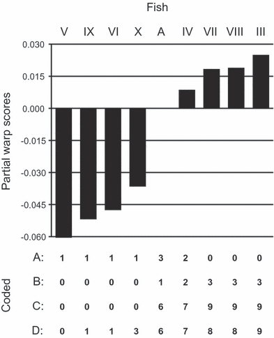
The second complaint against Naylor can be shown to miss the mark by just analysing Naylor’s data in various common ways, most of which result in the wrong tree. We show in Fig. 1 four different coding schemes, and they lead to four different topologies. Varying the analyses (like using distance methods and combining correlated characters) results in four more topologies. We reconsidered the way Naylor’s partial warps were coded and handled in the analysis, and this brings us to the first source of discomfort with his study—the quantity of data transformations and whether those have any bearing on reality. We agree that Naylor’s analysis required a number of steps, but it is here that we find the old study of continued interest and supportive of the latest work on morphometric phylogenetics. The critical mistakes in Naylor’s analysis were his coding of the partial warps, treating them as unordered, and his handling of character independence; once these are fixed, the original partial warp data lead exclusively to the true tree. Of course, arguing over the proper steps needed to transform morphometric data such that they can be used for phylogenetic analysis will irk those who dislike certain amounts or types of data transformations in phylogenetic analyses (see Crowe, 1994), or at least prefer them to be hidden in the bowels of user-friendly phylogenetic applications. However, our conclusion after looking more closely at Naylor’s analysis is that it supports the recent innovations made in TNT (Goloboff et al., 2006, 2008; Catalano et al., 2010; Goloboff and Catalano, 2010).

Given the phylogenetic programs of the day, Naylor needed to code his partial warps in order to analyse them phylogenetically, and he did so by giving all warps within 0.5 standard errors the same code and treating them as unordered. (There was a clerical error in the code for warp 19×, but it did not make a difference.) The resulting codes simply clustered together taxa that were most similar for certain partial warps, since, being unordered, different state codes contained little information about the magnitude of partial warp differences. Moreover, the codes appear to have been applied inconsistently, with some taxa receiving different states in spite of being more similar to each other than taxa receiving the same state (Fig. 1A). Ordering the codes (and treating them as ordered in the analysis) does not lead to the true tree, nor does a change in codes such that they capture the magnitude of the differences (while keeping Naylor’s like-coded taxa the same) (Fig. 1B,C, respectively). Only a coding scheme that follows Thiele’s (1993) gap-coding—where the partial warps are coded simply by rounding them to the nearest whole number after being standardized to the maximum value allowed by the program (here 0–9 in PAUP*)—results in a single parsimonious tree that is the true tree, and only when they were analysed as ordered (Fig. 1D). Zelditch et al. (2000) suspected that Naylor’s coding scheme could have been the source of problems, but they did not pursue the question nor point out the large amounts of information lost by treating the characters as unordered; upon reflection, Naylor’s coding was a radical transformation of the data.

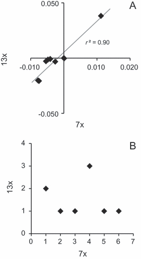
Gap-coding is appealing and popular, and since it roughly approximates continuous data, the obvious next step is to analyse the partial warp data as continuous (Goloboff et al., 2006). This, however, does not result in the true tree, which highlights the other problem with Naylor’s analysis, his handling of character independence. Naylor changed his simulated fish in different areas (like the tail or head) on different lineages, and this he hoped would lead to character independence and a lack of homoplasy. One of the disappointments of Naylor’s results was a high amount of homoplasy, as measured as the retention index (RI) on the shortest trees. However, partial warp calculations can interpret shape changes purposefully made in one body region as being the result of more efficient changes in another area or throughout the body. Thus, Naylor’s different transformations may have resulted in various changes and reversals in the same landmarks throughout the tree and thus homoplasy. In any case, tree quality does not relate to the amount of homoplasy (Goloboff, 1991), and the interesting aspect of the partial warp data is that homoplasy can be minimized by the true tree. Zelditch et al. (2000) correctly pointed out that Naylor should not have expected low homoplasy, although they appear to have confused homoplasy and independence, the latter of which was the real problem. They suggest combining each set of partial warps that changed on a branch into a different character, akin to using phylogenetic correlation to discover dependent characters, but their method would combine the same partial warps in different ways in the same analysis. MacLeod (2002) did his analysis of relative warps based on anatomical clusters, partially to capture Naylor’s attempt at insuring independence but also to generate enough coded characters at the end for phylogenetic analysis. Likewise, Goloboff and Catalano (2010) downweighted landmarks grouped by the authors into configurations. Both reanalyses of Naylor’s fish result in the true tree, and this may be due to their control of dependent characters, which do exist in Naylor’s data set. Partial warps 7× and 13× are tightly correlated, and when we combined them into one character, we found the true tree when analysing the data as continuous in TNT. In fact, making successive character combinations by lowering the threshold for dependence (de Bivort et al., 2010), the true tree was found when the data set was collapsed down to 69, 67–58 and 30 characters. One would never know that 7× and 13× were so highly correlated from Naylor’s original coding (Fig. 2), but apparently they contain enough misleading signal that the true tree cannot be found when it is duplicated and unaltered by gap-coding.

Capturing magnitude differences (by using continuous data or, at the very least, gap coding), maximizing character independence (through various techniques), avoiding anatomical structures most exposed to ecological selection pressures, and removing size information (not an issue with Naylor’s same-sized fish) are the key steps needed to capture phylogenetic signal and sideline extraneous processes in morpohometric data. Beyond that, different methods for analysing landmarks appear to be robust in capturing phylogeny, if not always practical or agreeable for different users. Moreover, they generate cladistic characters, since Naylor’s data, uncoded or coded in various ways, and with or without the collapse of dependent characters, lead to various wrong trees built using UPGMA and neighbour-joining. Only MacLeod’s coded data give the true tree using distance (specifically, neighbour-joining), but his characters were already a phenetic clustering of the fish by each body region. Rather than being a blot on the history of morphometrics in phylogenetics, Naylor’s simulation is ultimately in agreement with what we are learning about how morphometric data behave in phylogenetic analysis.