A deep active learning framework for mitotic figure detection with minimal manual annotation and labelling
Abstract
Aims
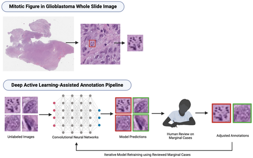
Accurately and efficiently identifying mitotic figures (MFs) is crucial for diagnosing and grading various cancers, including glioblastoma (GBM), a highly aggressive brain tumour requiring precise and timely intervention. Traditional manual counting of MFs in whole slide images (WSIs) is labour-intensive and prone to interobserver variability. Our study introduces a deep active learning framework that addresses these challenges with minimal human intervention.
Methods and results
We utilized a dataset of GBM WSIs from The Cancer Genome Atlas (TCGA). Our framework integrates convolutional neural networks (CNNs) with an active learning strategy. Initially, a CNN is trained on a small, annotated dataset. The framework then identifies uncertain samples from the unlabelled data pool, which are subsequently reviewed by experts. These ambiguous cases are verified and used for model retraining. This iterative process continues until the model achieves satisfactory performance. Our approach achieved 81.75% precision and 82.48% recall for MF detection. For MF subclass classification, it attained an accuracy of 84.1%. Furthermore, this approach significantly reduced annotation time - approximately 900 min across 66 WSIs - cutting the effort nearly in half compared to traditional methods.
Conclusions
Our deep active learning framework demonstrates a substantial improvement in both efficiency and accuracy for MF detection and classification in GBM WSIs. By reducing reliance on large annotated datasets, it minimizes manual effort while maintaining high performance. This methodology can be generalized to other medical imaging tasks, supporting broader applications in the healthcare domain.
Graphical Abstract
We propose a deep active learning framework for mitotic figure detection and classification in glioblastoma whole slide images. By iteratively selecting uncertain samples for expert review and model retraining, our approach achieves high accuracy while reducing annotation time by nearly 50%, demonstrating its potential for efficient cancer diagnosis.
Abbreviations
-
- CNN
-
- convolutional neural network
-
- CNNs
-
- convolutional neural networks
-
- COCO
-
- common objects in context
-
- GBM
-
- glioblastoma
-
- GM
-
- granular mitotic figure
-
- H&E
-
- Hematoxylin and Eosin
-
- mAP50-95
-
- mean Average Precision at Intersection over Union thresholds from 0.5 to 0.95
-
- MF
-
- mitotic figure
-
- MFs
-
- mitotic figures
-
- SGD
-
- Stochastic Gradient Descent
-
- TCGA
-
- The Cancer Genome Atlas
-
- UIP
-
- Unlabelled Image Pool
-
- WSI
-
- whole slide image
-
- WSIs
-
- whole slide images
-
- yolov8-cls-m
-
- YOLOv8 Classification Medium
-
- yolov8-m
-
- YOLOv8 Medium
Introduction
The quantification and categorization of mitotic figures (MFs) in histology slides is essential for the diagnosis and grading of cancers such as glioblastoma (GBM).1 It is not only important for grading, but it can also help guide treatment decisions.2 In general, MFs can exhibit either typical or atypical morphologies.2, 3 In particular, one subcategory of atypical MFs unique to GBMs is granular mitotic figures (GM). A high mitotic index (i.e. the proportion of cells undergoing mitosis) is often associated with a more aggressive phenotype and, subsequently, a poorer prognosis in many neoplasms.3
However, manually counting MF in haematoxylin and eosin (H&E) stained whole slide images (WSIs) requires expertise to differentiate MFs from morphological mimickers, such as lymphocytes, Creutzfeldt-Peters cells and apoptotic bodies. The task is further complicated by tumour tissue heterogeneity, processing artefacts and visual fatigue. In a traditional anatomic pathology service, a mitotic hotspot is visually estimated and at least 10 adjacent non-overlapping high-power fields are analysed for mitosis by a pathologist.4 This method of estimation or ‘eyeballing’ is efficient, but often overlooks the tissue heterogeneity and can miss MFs not included in the mitotic hotspots.
Advanced computational tools and deep learning models offer potential solutions by automating MF detection. However, they often require large labelled datasets to perform well. Creating sufficient and accurately labelled MF datasets is highly laborious.
To address these challenges, we developed an active learning framework that integrates two convolutional neural networks (CNNs) based on the YOLOv8 architecture.5, 6 We selected 66 H&E-stained GBM WSIs from The Cancer Genome Atlas (TCGA) as our unlabelled data pool. To begin, we manually labelled a small dataset with approximately 379 MFs to train the initial models. These models were then used to screen the remaining unlabelled WSIs, providing preliminary annotations. A tri-class thresholding strategy was applied to select MFs with ambiguous morphology from model-generated annotations for further review. Only the most challenging cases, flagged as marginal cases, were reviewed by pathologists and trained research assistants. This approach significantly reduced human effort. Selected marginal cases were prioritized in the model retraining process. The updated models were then used to provide initial MF annotations in the subsequent iteration, and this process continued iteratively.
Our annotation and detection pipeline, incorporated into the AI4Path web platform,7 requires no specialized training and can be accessed through any modern web browser. AI4Path further offers confidence threshold adjustments within each of the MF subclasses, allowing users to adjust model sensitivity for marginal MF cases. It also features precision-recall adjustments, enhancing its usability for pathologists.
Using this active learning framework, only less than 30% of the total MFs required manual review, as these were primarily ambiguous edge cases that were more time-consuming to annotate. Reviewing this smaller subset still took significant effort, but the framework ultimately reduced the total annotation time by half. Additionally, our models achieved near-optimal performance (within 15% of the best results) using only about 1000 marginal cases for training. In comparison, achieving similar performance with a non-active learning framework required approximately 2500 randomly selected training samples. The pipeline not only improves annotation efficiency but also reduces the challenging cases necessary for review. Prioritizing these marginal cases in model training also significantly enhances performance with much fewer samples.
This study presents a significant advancement in MF quantification for GBM WSIs, showcasing the potential of deep learning models integrated with active learning to improve diagnostic accuracy with minimal data and manual effort. Our method can be applied to other medical imaging tasks, making it useful in different areas of healthcare.
Methods
Dataset
In this study, 66 WSIs were retrieved from the TCGA GBM database, which included the most comprehensive data profiles (mRNA expression, methylation, etc.). Annotation data and genomic data were analysed in another project. Initially, two WSIs were selected based on typical morphological features observed in GBM and were manually annotated by pathologists, yielding 379 MFs for the initial training dataset. The remaining 64 WSIs were annotated using our active learning framework. During the CNN training and inference, WSIs were processed into 640 by 640 pixel patch images, discarding patches without MFs. Additionally, MFs were morphologically classified into normal, atypical and GM classes. These categories were unbalanced due to the natural occurrence rates of each MF subtype within GBMs.
Active Learning Framework
An overview of the active learning framework is illustrated in Figure 1. To start, 66 GBM WSIs were retrieved from the TCGA database, referred to as the Unlabelled Image Pool (UIP) for this study. Two WSIs were then selected from the UIP and manually annotated by 3 pathologists each, yielding 379 MF training samples used as the initial training dataset (L0). With samples from L0, we trained our first version of CNNs, which included one object detection model and one classification model.
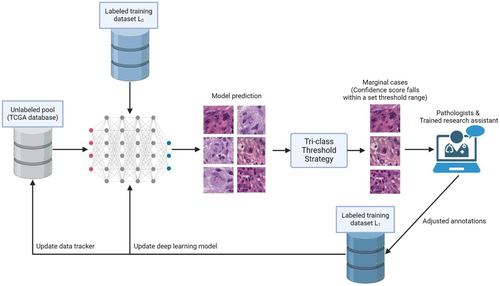
With the first CNNs ready, we began processing the remaining GBM WSIs in the UIP. Each WSI underwent our inference pipeline, and the results were filtered using a user-specified confidence threshold for each MF subclass (Tri-class Threshold Strategy). Cases with confidence scores falling within the specified range (0.500 to 0.725), likely indicating ambiguous morphology, were flagged as marginal cases. These marginal cases were then reviewed by pathologists or trained research assistants, while cases with high confidence were directly added to the labelled training dataset (L1) by default. Once the marginal cases were reviewed and categorized, they were eventually added to L1 with a designated tag.
During each iteration of the CNN's retraining process, flagged marginal cases were prioritized over randomly selected training samples. Over time, this approach improved the pipeline's performance in MF detection and categorization, reducing the manual annotation workload and resulting in more reliable outcomes.
Inference Pipeline
Due to the large size of WSIs (averaging 100,000 by 100,000 pixels in size), direct detection is computationally prohibitive, making preprocessing mandatory. Our inference pipeline splits WSI processing into two steps as shown in Figure 2. First, the WSI was compressed into a manageable size of around 1000 by 1000 pixels. An adaptive thresholding and morphological refinement algorithm generate a binary mask to differentiate tissue from the background.8 This created a 2D map where each element, represented by a binary value of 0 or 1 (0 indicating minimal or no valuable information and 1 indicating the opposite), corresponded to each patched image to be processed in the following step.
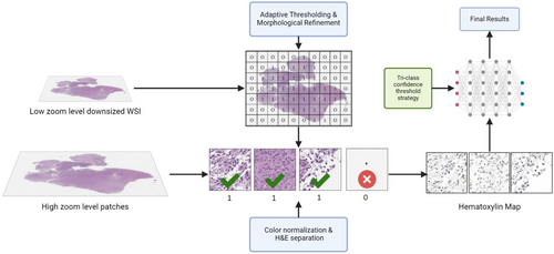
In the second step, the original WSI was processed into 640 by 640 pixel patches. Each patch image was then cross-checked against the 2D map generated in the first step to filter out those with minimal or no useful information. To address varying stain intensities and shades, the Stain Vector & Intensity Variation and Correction method was applied, which involves adjusting the colour vectors and intensities of stained tissue images to standardize and normalize the visual representation for consistent and accurate analysis, ensuring optimal experimental results.9 Furthermore, given the focus on nuclear material and the H&E staining of WSIs in our dataset (Haematoxylin primarily staining nucleic acid in the nucleus blue and Eosin staining cytoplasmic proteins pink), we performed H&E separation (as shown in Figure 3) to isolate and examine only Haematoxylin-stained nuclei.10 The processed patch images were then sent to our object detection and classification CNNs to obtain the final results.

Mitotic Figure Detection & Subtype Classification
As shown in Figure 4, a two-stage object detection and classification pipeline was implemented. Two CNNs with the YOLOv8 architecture were trained, one for detecting MF objects (Model A) and the other for classifying subtypes (Model B).6 The YOLOv8 medium (yolov8-m) model was used for object detection, while the YOLOv8 classification medium (yolov8-cls-m) model was used for subtype classification. Both models were initialized with pre-trained weights from the COCO dataset. To better address class imbalance in the classification task, we replaced the default entropy-based loss function with focal loss.11 No other structural modifications were made to the Ultralytics base models. Both models were trained for 50 epochs during initial training and in each retraining iteration, using the Stochastic Gradient Descent (SGD) optimizer for yolov8-m and the Adam optimizer for yolov8-cls-m.12, 13 To prevent overfitting, an early stopping mechanism was implemented with a tolerance set to 25 epochs.14 A batch size of 32 was chosen to optimally balance training speed and GPU memory constraints on the single RTX 4090, ensuring efficient resource utilization while maintaining convergence speed and generalization performance.15 To improve model robustness, training included standard data augmentation techniques such as random flips (horizontal/vertical), ±10° rotations, brightness/contrast adjustments and scale jittering.16 All other settings were kept as default from the Ultralytics YOLO library.6
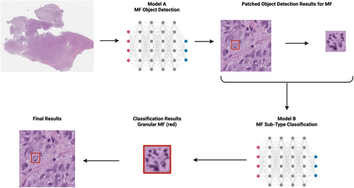
At first, patch images were fed into Model A to perform object detection, identifying MFs in the given images. Once all MFs were located, snapshots of each detected MF were taken and sent to the classification model, Model B, which morphologically classified them into three subtypes: normal, atypical and granular. The different phases of normal MF were not further delineated, due to the lack of clinical importance. Granular mitosis is a type of atypical MF, but was designated as a separate group in this study, because of their unique appearance and abundance in GBM samples. Detections were represented as bounding boxes. Using the coordinates of these bounding boxes and the patched images, we applied the results to the original WSIs, providing the final detection and classification outcomes.
Model Selection and Benchmarking
| Model | mAP50-95 | Inference time (per WSI) | Remarks |
|---|---|---|---|
| Faster R-CNN | 0.783 | 65.2 sec | Strong accuracy but slow inference |
| RetinaNet | 0.799 | 59.8 sec | Good balance, slower than YOLOv8 |
| YOLOv5 | 0.801 | 28.6 sec | Fast inference, decent accuracy |
| YOLOv8 | 0.823 | 30.1 sec | Best trade-off for accuracy and speed |
Each model was trained and evaluated on a subset of our pathologist-verified dataset using standardized training parameters: 50 epochs, batch size 32 and early stopping with a tolerance of 25. We evaluated mean Average Precision (mAP50-95) and inference speed per WSI.19
YOLOv8 demonstrated the best overall trade-off between detection accuracy and inference efficiency, making it well-suited for integration into real-time or large-scale annotation platforms like AI4Path.
AI4Path Web Portal
To enhance accessibility and collaboration, we have integrated our annotation and detection pipeline into a web-based platform.7 This platform is designed for various clinical applications, including Colon Polyp true/pseudo invasion classification, Ki-67 indexing, and several other useful features.20 In this study, we extended the platform's capabilities by incorporating the proposed active learning framework for GBM-related tasks as shown in Figure 5. This integration enables easy access for pathologists and researchers, facilitating the use of our active learning framework in real-world diagnostic settings.
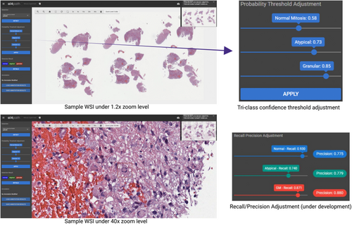
In object detection tasks, precision and recall are crucial metrics for evaluating a model's performance. Precision measures the accuracy of the positive predictions, while recall measures the model's ability to identify all relevant objects. Balancing these metrics ensures that the model accurately and comprehensively detects objects with minimal errors. To achieve this balance, a Precision & Recall adjustment feature was also incorporated into the annotation tool in the AI4Path web portal. This feature allows pathologists to manually balance these two metrics to ensure the most optimal results for specific use cases.
Results
TCGA Data Annotation
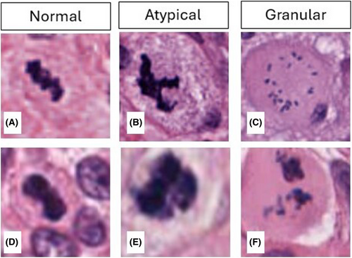
Our initial dataset comprised 66 GBM WSIs. Using the proposed deep active learning framework, the initial screening and annotations were performed. Pathologists and trained research assistants were only required to review marginal cases with uncertain morphology, which allowed them to efficiently annotate the entire set of 66 WSIs. Of these, 50 WSIs received further verification from at least one pathologist. As a result, 804 normal MFs, 728 atypical MFs and 1,955 granular MFs were annotated. Selected mitotic figures from each group are shown in Figure 6. The whole annotation dataset is available at GitHub (https://github.com/h26liu/gbm-db). The ambiguous cases are also included in the same repository.
Active Learning Performance
The focus of this study was to implement a deep active learning framework to accelerate the iteration of our CNNs and enhance the accuracy and efficiency of MF object detection and classification tasks.
As a result, our active learning approach offers several benefits. First, it reduces the amount of manual annotation required by pathologists by about 70%, as the model becomes more adept at handling common cases autonomously; only the most marginal cases require expert review. In our experiments, the time required to annotate all 66 WSIs were cut into half (estimated as over 900 min), compared to the manual annotation approach. Second, it accelerates the model iteration process, enabling quicker refinements and improvements. This results in consistently accurate detection and classification over time, even with significantly less training data.
We compared active learning to traditional passive learning using the same dataset, evaluating our MF object detection model with mAP50-95 and our sub-type classification model with accuracy.19 As shown in Figure 7a, the object detection model reached near-optimal mAP50-95 scores much faster with active learning (after 1000 training samples) than with passive learning (after 2750 training samples). Similarly, as shown in Figure 7b, the accuracy of the sub-type classification model reached approximately 80% more quickly using the active learning method (in fewer than 20 training iterations) compared to the passive learning strategy (around the 34th training iteration). The framework ensures the model is trained on the most challenging and informative cases, maximizing the effectiveness of manually labelled training data while maintaining nearly identical performance to the non-active, exhaustive labeling method.

These results demonstrated that the active learning framework significantly enhances the efficiency of the annotation process and makes annotating large datasets of high-resolution WSIs possible.
Model Accuracy
As mentioned earlier, we implemented a two-stage object detection and classification pipeline. To verify our method, we created a validation set using WSIs from the pathologist-verified cohort that were entirely separate from those used for training, ensuring no WSI-level overlap. Subtype proportions (normal, atypical, granular) were maintained. Training and internal testing were split at the patch level, which may result in patches from the same WSI appearing in both sets. Given the limited number of annotated WSIs, this was a necessary trade-off. We performed five-fold cross-validation on the independent validation set, and all reported metrics are averaged across folds. The final assessment of our MF object detection model showed strong performance, with average precision of 81.75% (±2.3%) and recall of 82.48% (±2.5%), demonstrating the method's effectiveness in accurately and comprehensively identifying MFs.
For the subtype classification model, we followed the same approach to create the validation dataset, ensuring it included only pathologist-verified samples, comprising approximately 10% of all annotated samples. Classification accuracy, calculated as the number of correctly classified images divided by the total number of images, was used as the evaluation metric. Results are reported as means ± standard deviations from five-fold cross-validation. The model achieved an average accuracy of 84.1% (±1.9%).
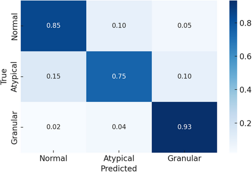
To further evaluate classification performance, we conducted a detailed error analysis. As illustrated in Figure 8, granular MFs were the most accurately classified, exhibiting minimal confusion with other subtypes. In contrast, atypical MFs demonstrated the highest misclassification rates, most frequently labelled as normal. This confusion likely stems from subtle morphological overlaps between atypical and normal MFs, underscoring the inherent challenge in distinguishing these two classes.
System Efficiency
Efficiency is a key factor when evaluating how practical an application is for real-world use. To determine the efficiency of our system, we tracked how long it took to perform object detection and subclass classification on our dataset of 66 WSIs. On average, our system processes a WSI in just 378 s (about 6.3 min). This is much quicker compared to the approximately 30–60 min typically needed by a pathologist to examine an entire WSI. As illustrated in Figure 9, we use the time spent detecting MFs in two WSIs as an example. It took pathologists 45 min to manually count 162 MFs in TCGA-08-0386 (DX1) and 60 min to count 220 MFs in TCGA-02-0033 (DX1). In comparison, our system completed the detection in just 0.8 and 5.7 min, respectively.
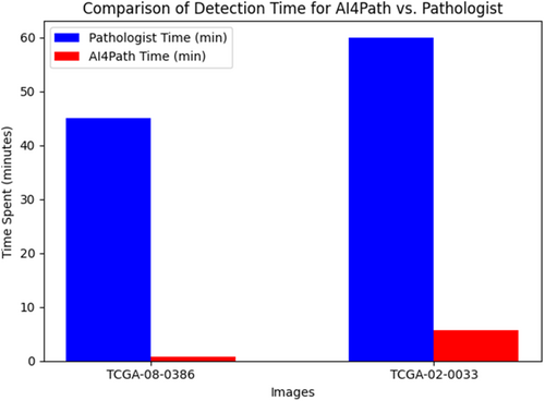
Moreover, the time required for a pathologist to review WSIs can vary widely due to factors such as slide complexity, experience level, visual fatigue from large caseloads and available resources. Ambiguous slides, in particular, may require several hours of review and consultation with colleagues. In contrast, our system's processing time depends only on the size of the tissue areas within a WSI and remains consistent regardless of other factors. This reliability ensures that our system streamlines the annotation process efficiently.
Discussion
Accurately counting MF is crucial for diagnosing and grading cancers. In the case of GBM, one of the most challenging brain tumours with dismal progression free survival and overall survival rates. MF indexing in GBM provides valuable insights into tumour growth, guiding the selection of the best treatment plan. However, manually counting MFs in WSIs is labour-intensive, and prone to inconsistencies due to visual fatigue and subjectivity.
With the advancement of deep learning, various computational tools have become available to assist in the MF indexing process. However, achieving satisfactory results typically requires a large amount of annotated data, necessitating extensive human effort. To address this, we designed and implemented an active learning framework powered by two CNNs: one for MF detection in WSIs and the other for MF subtype classification. We used H&E stained GBM WSIs from TCGA. After manually annotating a small dataset to train initial models, these models screened the remaining unlabelled WSIs. Our tri-class thresholding algorithm flagged only the most ambiguous MFs for review, while the rest were automatically added to the training set. Flagged cases were prioritized for model retraining, and the updated models provided annotations for the next iteration. This iterative process continued until satisfactory model performance was achieved, significantly reducing the manual review workload while maintaining model accuracy and iterative speed.
While our framework prioritizes manual review of marginal cases, a subset of high-confidence predictions was also manually verified in fully annotated WSIs by pathologists. However, due to time constraints, this verification was not performed across all WSIs. As a result, some high-confidence errors may have gone undetected. The current threshold range was selected empirically without formal calibration. In future work, we plan to explore confidence calibration and more dynamic thresholding methods to improve model certainty estimates and reduce potential error leakage.
To enhance accessibility, we integrated the proposed active learning framework into AI4Path. AI4Path requires no expertise to use and does not need heavy computational resources. It also includes handy features such as subclass threshold adjustments and precision-recall adjustments, making it user-friendly and efficient. Our research collaborators from institutions across Canada have seamlessly utilized AI4Path to manually detect mitotic figures in our training set, and have verified ambiguous mitotic figures in over 80 WSI. AI4Path provides customizable features such as MF hotspot analysis if pathologists would still like to utilize synoptic reporting of MF counts in accordance with the College of American Pathology electronic cancer protocols.
With the aid of the proposed framework, pathologists and research assistants only needed to review less than 30% of the total MF samples within select WSIs. This helped save almost half of the total annotation time (approximately 900 min) across the 66 WSIs in this study compared to the traditional approach. Additionally, our models achieved nearly identical results with less than half of the training samples (1000 out of 2500) required for non-active learning methods. This demonstrates that our framework significantly reduces the number of samples needed while maintaining excellent performance.
So far, 66 GBM WSIs have been annotated using our framework, with 50 verified by pathologists. In the MF detection task, our models achieved an average precision of 81.75% and a recall of 82.48% at a confidence threshold of 0.75, and a classification accuracy of 89.1% for normal, granular and atypical MFs in the subtype classification task. These results demonstrate the effectiveness of our approach in balancing precision and recall, thereby supporting the diagnostic process.
As we continue to collect additional WSIs and annotations, we aim to refine our models and extend the application to other cancer types. Our goal is to enhance diagnostic accuracy with less data and minimal manual effort, ultimately improving pathology workflows and patient outcomes.
In summary, our study presents a significant advancement in MF quantification for GBM WSIs, demonstrating the potential of deep learning integrated with active learning to improve diagnostic efficiency. Future work will focus on broadening the applicability of our approach and further optimizing its performance across various datasets.
Author contributions
E.L.: development of methodology, data analysis, original draft preparation; A.L.: data curation and analysis, original draft preparation; P.K. and Y.Z.: data curation, manuscript review and editing; B.W.: manuscript review and editing; C.L. and Q.Z.: project conceptualization, supervision, funding acquisition, manuscript review and editing.
Funding information
Pathology Internal Funds for Academic Development (PIFAD) of Western University (QZ); Western Dean's Office Research Opportunities Fellowship (DUROP) (AL).
Conflict of interest
The authors declare no conflicts of interest.
Open Research
Data availability statement
The images used in this study are publicly available from The Cancer Genome Atlas (TCGA) database. The annotations and corresponding metadata generated for this study are openly accessible at our GitHub repository: https://github.com/h26liu/gbm-db.


