Marine invertebrate migrations trace climate change over 450 million years
Funding information: VolkswagenStiftung; Deutsche Forschungsgemeinschaft, Grant/Award Number: KI 806/16-1 and KO 5382/1-1
Abstract
Aim
Poleward migration is a clear response of marine organisms to current global warming but the generality and geographical uniformity of this response are unclear. Marine fossils are expected to record the range shift responses of taxa and ecosystems to past climate change. However, unequal sampling (natural and human) in time and space biases the fossil record, restricting previous studies of ancient migrations to individual taxa and events. We expect that temporal changes in the latitudinal distribution of surviving taxa will reveal range shifts to trace global climate change.
Location
Global.
Time period
Post-Cambrian Phanerozoic aeon.
Major taxa studied
Well-fossilized marine benthic invertebrates comprising stony corals, bivalves, gastropods, brachiopods, trilobites and calcifying sponges.
Methods
We track deviations in the latitudinal distribution of range centres of age boundary crossing taxa from the expected distribution, and compare responses across latitudes. We build deviation time series, spanning hundreds of million years, from fossil occurrences and test correlations with seawater temperature estimates derived from stable oxygen isotopes of fossils.
Results
Seawater temperature and latitudinal deviations from sampling are positively correlated over the post-Cambrian Phanerozoic. Simulations suggest that sampling patterns are highly unlikely to drive this putative signal of range shifts. Systematically accounting for known sampling issues strengthens this correlation, so that climate is capable of explaining nearly a third of the variance in ancient latitudinal range shifts. The relationship is stronger in low latitude taxa than higher latitude taxa, and in warm ages than cool ages.
Main conclusions
Latitudinal range shifts occurred in concert with climate change throughout the post-Cambrian Phanerozoic. Low latitude taxa show the clearest climate-migration signal through time, corroborating predictions of their shift in a warming future.
1 INTRODUCTION
The movement of species to previously colder areas may be the most dependable response of organisms to climate warming (Chen, Hill, Ohlemüller, Roy, & Thomas, 2011; Parmesan & Yohe, 2003; Poloczanska et al., 2013). While fine-scale range shifts responding to regional climate change are not always directed poleward (Burrows et al., 2014), in the oceans, climate-induced latitudinal shifts (‘migrations’ henceforth) are already dramatic (García Molinos et al., 2016; Sorte, Williams, & Carlton, 2010). Poloczanska et al. (2013) observed an average rate of 72 km/decade at which poleward range edges expand, although the movement of centroids is only half of that, mostly because trailing edge contractions are still moderate. Nevertheless, these migrations indicate that even modest changes in global sea surface temperature (0.07 °C/decade; Burrows et al., 2011) can have dramatic effects on the latitudinal distribution of marine animals. Marine ectotherms are expected to track coherently their thermal limits (Sunday, Bates, & Dulvy, 2012), especially because their thermal niches are generally conserved over macro-evolutionary time-scales (Saupe et al., 2014) and there are hard limits to adaptation (Storch, Menzel, Frickenhaus, & Pörtner, 2014). However, rates of migrations vary among species and higher taxa such that communities are unlikely to migrate cohesively, changing community composition (Graham et al., 1996; Valentine & Jablonski, 1993; Walther et al., 2002). Consequently, this redistribution of biodiversity is expected to alter ecosystem functioning and, thereby, human well-being (Pecl et al., 2017). Therefore, the separation of general and contingent aspects of biodiversity responses to climate warming is a key goal for ecologists, enabling confident prediction of future developments.
The current expected magnitude, and perhaps even rate, of warming may not be without equal in the Phanerozoic aeon (Kemp, Eichenseer, & Kiessling, 2015; Zachos, Dickens, & Zeebe, 2008; but see Foster, Royer, Lunt, Olsen, & Beerling, 2017). Organisms have endured global cooling intervals lasting several millions of years (Royer, Berner, Montañez, Tabor, & Beerling, 2004) and shorter intervals of excessive tropical heat (Song et al., 2015; Sun et al., 2012), both forced partly by atmospheric CO2 (Foster et al., 2017; Royer, 2006). Tropical taxa may be the most responsive to long-term climate warming because high development rates enable rapid responses (Walters, Blanckenhorn, & Berger, 2012). They also often live close to maximum thermal limits set by phylogeny (typically < 35 °C, never exceeding 45 °C for metazoans; Song et al., 2015; Storch et al., 2014; Walther et al., 2002). In response to climatic stressors, studies show examples of fossil taxa ostensibly migrating by latitude both for near time (e.g. Greenstein & Pandolfi, 2008; Kiessling, Simpson, Beck, Mewis, & Pandolfi, 2012; Roy, 2001) and deep time (e.g. Blois & Hadly, 2009; Martin-Garin, Lathuilière, & Geister, 2012; Thibault & Gardin, 2010). However, the consistency of global biodiversity responses to warming events is unproven. The fossil record is unique in its capacity to record how organisms responded to such ‘natural experiments’ of the past. Yet, numerous issues exist regarding the temporal and palaeo-geographical precision of fossil occurrences, which can distort evidence for global ecological patterns in deep time (e.g. Clapham & James, 2012). Spatio-temporal biases in sampling are the main driver of patterns in the fossil record and need handling correctly in order to identify ecological patterns (Vilhena & Smith, 2013).
Here we analyse the link between net latitudinal range shifts of marine invertebrates from geological age-to-age and seawater temperature. This scale emphasizes long-term net migration in response to long-term climatic processes. The effect on range shifts due to processes operating at finer scales, such as Milanković cycles, are thus averaged out. We expect latitudinal range shifts, either of individual fossil taxa or else averaged over many, to track global climate change, which we quantify independently. We expect this relationship to be clearest in low latitude taxa during relatively warm ages, as these taxa often live close to metazoan thermal maxima and warm global climate intervals may have forced many taxa to vacate the tropics. Three factors anticipated to affect the clarity of range shifts are the median occurrence latitude, number of sampled taxa and extinction rate. The first concerns which taxa are used to characterize the proxy for range shifts, while the second and third concern the observed number of taxa that could shift their ranges.
2 MATERIALS AND METHODS
2.1 The database
We downloaded occurrence data of fossil marine invertebrates on 8 February 2017 from the most comprehensive dataset of fossil metazoans currently available to science, the publicly-accessible Paleobiology Database (https://paleobiodb.org/). This used the standard download protocol except it excluded genera identified with some degree of uncertainty (‘aff.’, ‘cf.’, ‘?’). These data have their palaeo-coordinates calculated based on the GPlates plate tectonic model (Wright, Zahirovic, Müller, & Seton, 2013). Fossil collections were binned by their central age estimate to one of 94 geological ages (Gradstein, Ogg, Schmitz, & Ogg, 2012), averaging 6.12 Ma in duration. Collections with age uncertainties greater than the longest age duration (> 19.5 Ma) were removed. Similar to comparable studies of ancient geographical ranges (Foote, 2014), we assess range shift patterns at the genus level. This taxonomic level is a compromise between uncertainty in the species level taxonomy of fossils and data loss at coarser taxonomic resolutions (Valentine, 1974). Furthermore, species-level information is inconsistent and sparse in the Paleobiology Database and species longevities are typically below our temporal resolution. Duplicate genus occurrences per collection were removed to make collections more comparable (i.e. between collections with species level identified or not identified).
We included marine benthic invertebrate classes with good fossil records owing to their heavily calcified body parts, including stony corals, bivalves, gastropods, brachiopods, trilobites and sponges such as Stromatoporoidea. The Cambrian and older periods were removed because of sparse temporal and geographic coverage of both occurrence and climate proxy records. After filtering, 458,000 occurrences in 76,000 collections were available for analyses.
2.2 Sampling and taxa location shifts
We initially conceived various candidate proxies for ancient taxon range shifts. Initially, these included tracing age-to-age changes in surviving genus (i.e. that occurred in the previous age and the focal age) palaeolatitude, by range edges or centre, corrected for changes in sampling (occurrence) patterns (details in Supporting Information Appendix S1). Briefly, we concluded that data for specific genera may be too noisy to track across ages. Although range shifts are expressed at the individual genus level, a net range shift approach is required to overcome sampling inconsistencies and random noise. Therefore, we decided to average their range centres per age, rather than the age-to-age changes in them, maintaining our focus on survivors. The time series variance of median fossil genus range centres or edges is always dominated (R2 > .9) by sampling patterns (human and geological; Figure 1a and Supporting Information Appendix S2; also see Clapham & James, 2012). Therefore, we accepted sampling as the dominant driver of range shift patterns (Supporting Information Appendix S3 for further justification; cf. Powell, 2009; Vilhena & Smith, 2013). All candidate proxies for fossil range shifts were assessed by backward selection, based on Akaike information criterion (AIC) values, with median occurrence latitude, temperature and shifts in occurrence median latitudes as predictor variables. The occurrence distribution and individual distributions of fossil genera per age were typically skewed and multimodal so we decided a priori to use the median rather than the mean. Throughout most of the Phanerozoic, the northern palaeo-hemisphere is the best sampled (Figure 1; Vilhena & Smith, 2013) and thus we test our hypotheses on this hemisphere.
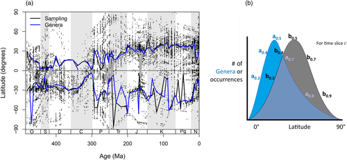
The palaeolatitudinal distribution of fossil occurrences (a) through the post-Cambrian Phanerozoic and (b) a schematic of how this is used to calculate the ‘latitudinal deviation’. (a) Each occurrence (n = 469,000) is shown as a black dot by its central age estimate. Global (grey line) and per hemisphere (black lines) trends are shown by median occurrence palaeolatitudes binned to geological ages and plotted at their mid-points. Blue lines show the median latitudinal range centre of genera per hemisphere (blue line minus black line gives the genus latitudinal deviation from sampling focus). Timescale after Gradstein et al. (2012); geological periods (shaded) are abbreviated along the x axis: O = Ordovician; S = Silurian; D = Devonian; C = Carboniferous; P = Permian; Tr = Triassic; J = Jurassic; K = Cretaceous; Pg = Palaeogene; N = Neogene. A hypothetical time slice, i, from (a) is shown in (b) for a single hemisphere to illustrate calculation of median and other latitudinal deviation quantiles. Note latitude is on the y axis in (a) and x axis in (b). In blue is a hypothetical distribution of genus range centres, a, of which any quantile can be calculated, the median being the .5-quantile. In grey is a hypothetical distribution of occurrences, b. For whichever quantile chosen, a – b gives the deviation of observed genus range centres from the ‘expected’ range centre, termed the ‘latitudinal deviation’
Global temperature was selected as an explanatory variable only for one candidate proxy (Supporting Information Appendix S2). This was the deviation of ai, the median of genus latitudinal range centres in time slice i, from bi, the median latitude of occurrences in time slice i (also termed sampling ‘centre’ or ‘focus’; Figure 1b). Here, b represents the null-expected median range centre of genera. Thereby, ai – bi is henceforth termed the ‘latitudinal deviation’ and a time series is built. This proxy is equivalent to the residuals from a regression. To maximize this proxy's effectiveness, we are interested in contrasting sampling bias (via b, the occurrence distribution) against ecological patterns (via a, the median genus range centres), so that the latitudinal deviation (a – b) represents bias-corrected ecological signal. b should therefore aim to represent the spatial biases as best possible, which we hypothesize is by the following steps. Supporting Information Appendix S2 discusses further how a latitudinal deviation time series describes genus range shifts from age to age.
To calculate genus range centres, a, we used only those genera that were sampled in two consecutive ages (bin-to-bin survivors, which were thus able to migrate). Furthermore, in an attempt to homogenize geographical sampling coverage between consecutive ages (i.e. sampling effort), we used matching cells to calculate a (Kiessling & Kocsis, 2016). Genus range centres were thus calculated from occurrences in only those geographical cells that were sampled in both consecutive time intervals. Grid cells were equal-area hexagons constructed using the R package icosa (Kocsis, 2017), with a mean cell area of 794,000 km2. Genus range centres were calculated separately for the Northern and Southern Hemispheres, to minimize inter-hemispherical differences (e.g. sampling coverage, genus ranges, regional climatic phenomena, continental shelf availability; Figure 1a). The Southern Hemisphere values were useful to supplement intervals when the Northern Hemisphere is poorly sampled (see below). To calculate sampling latitude, b, we used all marine fossils in our dataset, including stratigraphical singletons and without matched cells. Median sampling latitude was uncorrelated with climate (always p > .2; Supporting Information Appendix S4).
To assess differences in range shift responses between lower and higher latitude genera, we investigated different quantiles of the distribution of survivor latitudinal range centres per age, in addition to the median (quantiles in steps of .1, Figure 1b). These were used to calculate quantile latitudinal deviations following the previous approach, by adjusting the genus range centre quantile by the appropriate quantile of the sampling distribution for a time slice. For example, the .2-quantile of sampling latitudes was subtracted from the .2-quantile of genus latitudes to provide the .2-quantile latitudinal deviation (a.2-quantile – b.2-quantile). Time series of each quantile could thus be correlated with temperature. We modelled the behaviour of these quantile deviations (Supporting Information Appendix S5) and found that their correlations with independent climate data can be compared without problem. We also directly investigated sampling focal latitude as a source of error on latitudinal deviations. Standardizing variances of both occurrence time series and range centre time series, for each quantile separately, had little effect on quantile latitudinal deviations and their correlations with temperature (Supporting Information Appendix S5).
Inspection of Figure 1 suggests that the signal of climate-induced range shifts might be refined further by addressing particular sampling biases (listed 1–3). The global sampling focus drifts through time with the tectonic movement of the well-sampled modern-day Europe and North America, into the Southern Hemisphere prior to the Permian (Figure 1, grey line). Therefore (1) The Northern Hemisphere number of surviving genera was sometimes low (< 100, Supporting Information Figure S1). Switching the focal hemisphere, that is, replacing deviations in one hemisphere with those of the other, was systematically and automatically explored by setting thresholds for a minimum number of surviving genera, from one to 200. Thus, ages with surviving genera numbers below this threshold would switch to the other hemisphere to calculate deviations. The effect of this hemisphere switching was quantified for both hemispheres separately. (2) Across the post-Cambrian Phanerozoic, the median sampling latitude was 27.8° but it distinctly rose from the late Triassic onwards (Supporting Information Figure S2, absolute medians before late Triassic = 20.2°, after = 34.5°). We expected this rise to weaken the signal of climate induced range shifts, following our hypothesis that low latitude taxa should show clearer migratory responses to climate. Therefore, to maintain a low latitude sampling focus, we made a time series integrating the median with the strongest-related lower latitude quantile, using the former in ages when sampling focus was tropical (median sampling latitude < 23.4°) and the latter when the median sampling latitude was subtropical or higher (> 23.4°). This decreased the median palaeolatitude of genus occurrences to 19.9°. (3) We expected higher extinction rates to decrease the signal of climate-induced range shifts. We therefore used a weighted correlation test (see Statistical analysis). There is less than 1% chance that the climate-deviation correlation strengths resulting from the above refinements were caused by random entry of new collections (or < 6% chance for Northern Hemisphere only; Supporting Information Appendix S4).
2.3 Climate proxy data
To reconstruct temperature change over time, we use arguably the best available proxy for ‘deep time’: the δ18O values of well-preserved calcareous shells (but see Ridgwell, 2005; Royer et al., 2004). We downloaded the whole surface water (mixed layers < 300 m deep) oxygen isotope dataset of Veizer and Prokoph (2015). Oxygen stable isotope measurements from well-preserved calcareous fossils are traditionally used to reconstruct seawater temperatures but the oxygen isotopic composition of seawater needs to be known (Veizer & Prokoph, 2015). To adjust for the long-term trend in oxygen isotopic composition of seawater, we follow Veizer and Prokoph (2015) and detrended the time series using the equation: δ18Opw(‰) = −0.00003‰ t2 + 0.0046‰ t, with pw being Phanerozoic seawater in standard mean ocean water (SMOW) and t being age in Ma. For any given age, spatial variation in the oxygen isotopic composition of seawater, such as that attributable to salinity and pH variation (Grossman, 2012; Ridgwell, 2005), is expected to contribute mostly to variance rather than mean estimates (Veizer & Prokoph, 2015). Variation attributable to ice volume is relatively minor and relates to climate (Veizer & Prokoph, 2015). Tropical (including subtropical) records dominate the Veizer and Prokoph (2015) dataset (75% of all records). To optimize the representativeness of these data to the habitat of genera in our dataset, we only use data from tropical and subtropical palaeolatitudes. However, during the whole Jurassic Period to the Barremian age, when temperate isotope records dominate (Supporting Information Figure S3), we averaged temperate, subtropical and tropical records to ensure there was sufficient data over which to average. We binned isotope data to geological ages and computed their medians. The Induan age is not represented by any samples in this dataset so its temperature was interpolated between neighbouring age medians. We translated δ18O into degrees Celsius in all cases, using the transfer function in Visser, Thunell, and Stott (2003; recommended in Veizer & Prokoph, 2015), representing low latitude upper layer seawater.
2.4 Statistical analysis
Unless otherwise noted, hypothesis testing is based on nonparametric statistics such as Spearman's rho. Autocorrelation of time series data was removed using generalized differencing (McKinney & Oyen, 1989) [Δx = xi – rA(xi–1), where i is the time interval and rA the lag 1 autocorrelation coefficient]. We employed a moderate smoothing of latitudinal deviations and temperature using a symmetrical moving window of three consecutive bins for analysis, unless otherwise noted. This approach dampens the influence of various sources of error, including sample temporal accuracy, global representativeness and coverage of sampling distribution, and emphasizes long-term changes. Bootstrapped 95% confidence intervals (CIs) around the latitudinal deviation were calculated by resampling with replacement, for a from the list of genera range centres per age and for b from the occurrence latitudes per age. We performed 10,000 resamples and extracted the .025 and .975 quantiles from the distribution of a–b. The 95% CI time series are smoothed, as above. Ages that were more influential to the correlation tend to have narrower CIs (Supporting Information Appendix S2). Weighting of the correlation (package wCorr) was by inverse per capita extinction rate, uncorrected for age duration (Foote, 2000; smoothed, as for the other data), with all other details remaining the same as before. To investigate the relationship between sampling focal latitude and genus latitudinal deviation, we compare least squares regression slopes where residuals are approximately normal. This used the Z-statistic calculation, Z = b1 – b2/√(
 +
+
 ), where b1 is the regression slope of sample set 1 and SEb1 is the standard error of that slope (Cohen, Cohen, West, & Aiken, 2003). All analyses were performed in the R statistical computing environment (R Development Core Team, 2017).
3 RESULTS
3.1 Latitudinal deviations as climate-induced range shifts
Genus median latitudinal deviations of the better-sampled northern palaeo-hemisphere are positively correlated with seawater temperature across the post-Cambrian Phanerozoic (rho = .30, p = .01; Figure 2). This supports our hypothesis of linked climate change and latitudinal range shifts, although further validation of the potential signal is desirable to support, or deny, its existence. We anticipated three factors to affect clarity of the signal: (a) systematically supplementing the Northern Hemisphere latitudinal deviations with occurrences from the Southern Hemisphere when the number of sampled surviving genera became low vastly increased the correlation to rho = .48 (95% CIs = .29–.64, optimum threshold = 108 genera, Figure 3). The Southern Hemisphere remained uncorrelated with climate (Figure 3), even when restricted to the well-sampled Palaeozoic (rho = .22, p = .2). Additionally, (b) when the Northern Hemisphere median occurrence palaeolatitude vacated the tropics (> 23.4°; Supporting Information Figure S2), this vacation was corrected for by integrating the .2-quantile deviation, transcending the Northern Hemisphere correlation strength of either the median or .2-quantile alone with climate (rho = .40, 95% CIs = .19–.57). However, combining these two steps, (a) and (b), led to no further improvement in the correlation strength (rho = .40, 95% CIs = .19–.57, Figure 4). Finally, (c) weighting the correlation from step (a) (the highest so far) by age inverse extinction rate increased the correlation strength between seawater temperature and genus latitudinal deviation further (rho = .56, 95% CIs = .39–.70). The substantial increase in the correlation strength achieved by considering these a priori factors supports the validity of the latitudinal deviations as revealing ecological signal. Exploring the contribution of individual taxa to the correlation between temperature and latitudinal deviation suggests brachiopods to be particularly important (Supporting Information Appendix S6).
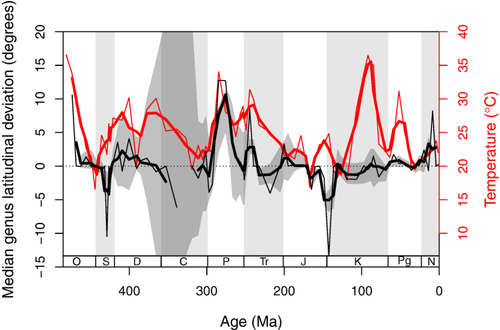
Latitudinal range shifts of Northern Hemisphere marine genera (black lines) are correlated with low latitude mean shallow seawater temperature (red lines, right-hand y axis). Temperature calculated from fossil shell oxygen isotopes following Veizer and Prokoph (2015). Grey shading around the thick black line shows bootstrapped 95% confidence intervals. For both variables, thick lines show a moving window of three consecutive bins. Thin lines show the unsmoothed bin-to-bin changes. Contributing genera median range centre = 24.6°. Geological periods are lightly shaded and abbreviated as in Figure 1. The gap in the latitudinal deviation time series shows a lack of occurrences for the Northern Hemisphere in one age. Latitudinal deviation mean is 0.32° (absolute mean = 1.93°). O = Ordovician; S = Silurian; D = Devonian; C = Carboniferous; P = Permian; Tr = Triassic; J = Jurassic; K = Cretaceous; Pg = Palaeogene; N = Neogene
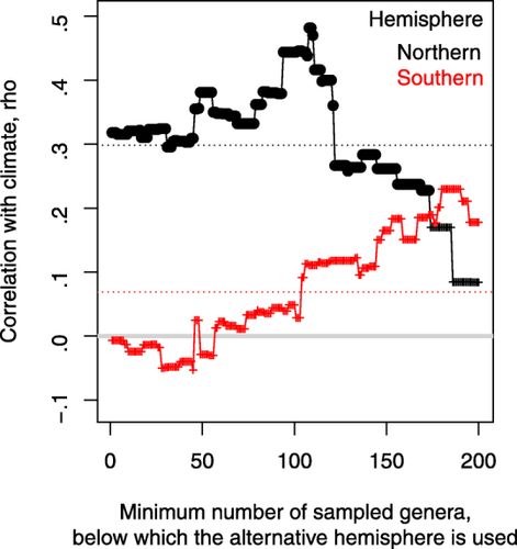
The effect of changing a threshold minimum number of genera in ‘hemisphere switching’ on the correlation of latitudinal deviation with climate. When the minimum threshold is reached, latitudinal deviations are sourced from the opposite hemisphere. Dotted lines show the correlation without any hemisphere switching, for northern and southern palaeo-hemispheres separately. Filled circles are p < .05. Serial autocorrelation in times series removed by generalized differencing
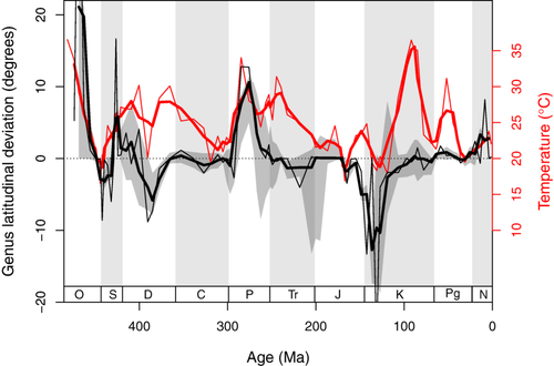
Time series of latitudinal range shifts of marine genera (black lines) improved by hemisphere switching alongside low latitude shallow seawater temperature (red lines, right-hand y axis). Details as in Figure 3. Contributing genera average a range centre of 27.6°. Latitudinal deviation mean is 0.54° (absolute mean = 3.10°). O = Ordovician; S = Silurian; D = Devonian; C = Carboniferous; P = Permian; Tr = Triassic; J = Jurassic; K = Cretaceous; Pg = Palaeogene; N = Neogene
3.2 Low versus high latitude genus responses to climate change
Genus latitudinal distribution quantiles vary systematically in their latitudinal focus such that the .1- and .2-quantiles tend to represent palaeotropical taxa, having median range centres of 12.5° and 16.2°, respectively. Higher quantiles represent higher latitude taxa, with median range centres up to 41.4° for the .9-quantile. Latitudinal deviation quantiles generally show an increase in strength of relationship with climate from higher to lower quantiles (rho = –.78, n = 9, p = .02; Figure 5; quantiles without hemisphere switching). 95% CIs around the correlation coefficient overlap zero for higher latitude taxa with range centres > 24.5°, although .8- and .9-quantiles appear particularly susceptible to random noise (Supporting Information Appendix S5).
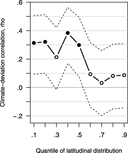
Correlation strength between shallow seawater temperature and genus latitudinal range shifts decreases from more equatorward (.1-quantile, median palaeolatitude = 12.5°) to poleward genera (.9-quantile, median palaeolatitude = 41.4°; quantile steps of .1). Solid symbols show Spearman's rho coefficients that 95% confidence intervals (dashed lines) overlap zero. Serial autocorrelation in times series removed by generalized differencing. The strongest correlation is with the .4-quantile (rho = .38, p = .001)
The latitudinal focus of occurrences changes over time, which permits an alternative test of differences in magnitude of latitudinal deviation between low and high latitude taxa. The magnitude of latitudinal deviation is significantly and negatively related to sampling latitude (rho = –.34, p = .002, unsmoothed data, Figure 6), such that sampling foci at lower latitudes more consistently show larger and positive (i.e. poleward) genus latitudinal deviations. When warm and cool ages are analysed separately, warm ages contributed more to the negative relationship between focal latitude and observed deviation, with significantly different warm and cool age regression slopes (Z-statistic = −2.65, p = .004; Figure 6a). The effects of sampling latitude and temperature on latitudinal deviation are largely independent (Figure 6b).
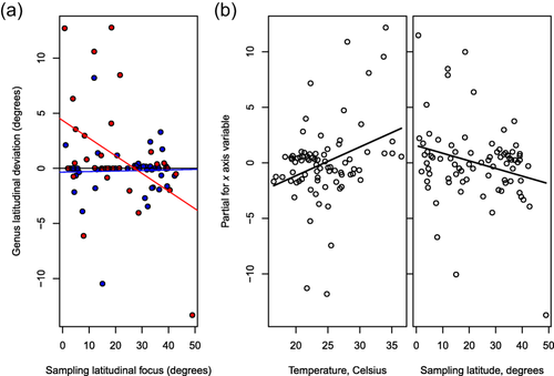
Poleward migrations are more likely to be recorded by lower latitude sampling foci, (a) especially during warming ages (red line and points, age seawater temperature > Phanerozoic mean, slope = −0.16, p = .01, n = 34). Each point represents one geological age. Blue line and points represent cool ages (age seawater temperature < Phanerozoic mean, slope = 0.005, n.s., n = 47). (b) Termplots of the independent effects of the predictor variables in a multiple regression including both temperature and sampling latitude as predictor variables for latitudinal deviations. Points are the partial residuals
4 DISCUSSION
Latitudinal deviations for marine invertebrate genera consistently trace global changes in seawater temperature throughout the post-Cambrian Phanerozoic. Global temperature explains up to 31.4% of the variance in putative range shifts (by rho squared, the variance shared between ranked variables), which is even more than observed for recent marine organisms (11% of variance, Poloczanska et al., 2013). This is strikingly high given the dating issues in both fossil occurrence and climate proxy data. Simulations of sampling biases (Supporting Information Appendix S4) suggest that this correlation is highly unlikely to emerge from sampling. Thus, we interpret genus median latitudinal deviations as indicating genuine range shift trends of fossil marine taxa. Low latitude taxa exhibit especially predictable migratory responses to climate warming. Fossils thus have great potential to elucidate ancient climate change and to help anticipate the effects of modern climate warming.
Perhaps our clearest result is the reliability of lower latitude taxa to respond to climate warming by poleward range shifts. In particular, the disproportionate strength of correlation of the .1-quantile with climate (versus the absence of correlation of even the .6-quantile) is striking, because the fringe quantiles (.1, .8 and .9, generally right-skewed distributions) are expected to be more biased by sampling constraints (edges) and therefore statistically noisier (Supporting Information Figure S4). Climate-range shift agreement is increased when sampling focal latitude is constrained to lower latitudes, here using a median–.2-quantile hybrid of latitudinal deviations. Tropical warming may then force regional range shifts (Walther et al., 2002) and even tropical extirpation of some species (e.g. Kiessling et al., 2012), which may live close to their phylogenetic maximum thermal limits (Song et al., 2015; Storch et al., 2014). Perhaps most importantly, temperature isotherms locally move at different speeds, or ‘climate velocities’, across the Earth's surface, and are expected to be higher at low latitudes, especially in marine habitats (Burrows et al., 2011). Poleward ‘pushes’ of taxon ranges may have been common in the past, when latitudinal diversity peaks (of a hemisphere) often did not fall upon the equator (Powell, 2009), and tropical species may be well adapted to track ‘pushes’ (Walters et al., 2012). Still, current migration patterns are more prevalent at the leading (poleward) edge than at the trailing edge (Poloczanska et al., 2013), suggesting a prevalence of species ‘pull’ forces arising from new climate opportunities. Marine species track closely their thermal niches (Sunday et al., 2012), such that ‘push’ forces may become just as strong as warming advances. Our study thus suggests that the most reliable impact of climate warming on species distributions still lies ahead.
We found no evidence for consistent climate-induced range shifts of higher latitude taxa, but we suggest that this is only because the signal is less clear, not because they are less affected by climate (Peck, Webb, & Bailey, 2004; cf. Powell, Moore, & Smith, 2015). High latitude genera also appeared to have no greater sensitivity to long-term cooling than lower latitude taxa. Perhaps this is because our seawater habitat temperature proxy focusses on low latitudes (Supporting Information Figure S3). Higher sampling latitudes do show equatorward migrations but this tendency is expected by chance (non-directed random migrations), given greater habitat area toward the equator (e.g. Jablonski et al., 2013). Higher latitude genera are far more volatile than lower latitude taxa (Supporting Information Figure S4), with some volatility attributable to real migrations (Powell et al., 2015) and some to proximity to the occurrence distribution edges. Higher latitude taxa endure seasonal fluctuation extremes, while regional climate changes, such as caused by the disruption of ocean currents or ice formation, may complicate migratory responses (Tingley, Koo, Moritz, Rush, & Beissinger, 2012). Therefore, higher latitude taxa may change latitude for many reasons other than changes in average global climate.
Short-term climate change related extinction events, where taxa are unable to track their thermal niche, may partly explain a weak observed climate–migration link. Weighting the time series by inverse extinction rate raised the climate–migration correlation strength. Temporal as well as regional extinctions may add noise to the data, with the lower number of surviving genera more influenced by random fluctuations. Extinction rates may also vary by latitude, depending on temporal interval (e.g. Kiessling & Aberhan, 2007; Powell et al., 2015). A modelling study suggests that extinction may be more likely a response by temperate species compared with tropical ones, as development rates may offset risks associated with being a thermal specialist (Walters et al., 2012). Consequently, extinctions may add another element obscuring climate-induced migrations of higher latitude taxa. The big five ancient mass extinctions of Raup and Sepkoski (1982) did not have a consistent effect on overall latitudinal migrations, perhaps because their hypothesized causes were diverse and their temporal durations far briefer than our temporal scale.
Averaging across our age-to-age absolute migrations over the 450 million years gives between 3–9 × 10⁻⁵ km/decade, depending on the quantile, which is five orders of magnitude lower than the average 31 km/decade observed over the last 60 years (Poloczanska et al., 2013). However, distances given by latitudinal deviations are not expected to be large. Firstly, latitudinal deviation is a relative measure of distance from the sampling centre to the median of genus range centres (Supporting Information Appendix S2). Secondly, genus range shifts integrate the somewhat chaotic dynamics of potentially many constituent species ranges. Thirdly, longer duration studies systematically underestimate rates. There is a negative power-law relationship between the timespan of observation and the observed rate of change both in evolutionary patterns and in rates of climate change (Gingerich, 2009; Kemp et al., 2015). This relationship is due to transient switchbacks in climatic trends for which there is ample evidence in palaeoclimates, even within intervals considered relatively stable (e.g. mid-Cretaceous; Wilson & Norris, 2001). Therefore, the potential of prehistoric species to change latitudinal positions over timeframes comparable with recent studies is critically underestimated.
The most prominent agreements between the time series of migrations and seawater temperature were around the cool intervals of the end-Ordovician and the Permo-Carboniferous (Royer et al., 2004), both with subsequent poleward pulses (hemisphere switching time series). Strong warming in the Early Triassic epoch (Sun et al., 2012; Song et al., 2015) drove poleward migrations of all Northern Hemisphere lower latitude quantiles (.1–.5), both in age-to-age and multi-age (smoothed) series. However, large changes in sampling distribution may weaken the ability of taxa deviations to describe real migrations, such as for the Southern Hemisphere Mesozoic and Cenozoic eras. We suggest that some parts of the fossil record (e.g. Early to Mid-Permian and mid-Cretaceous warming) are more reliable for detecting migration patterns than others (Clapham & James, 2012, for migration patterns of the Southern Hemisphere Permian; Ridgwell, 2005, for Phanerozoic intervals where oxygen isotopes become less reliable). In particular, mass extinction events severely decrease the number of surviving genera available to inform analyses of migration (e.g. Supporting Information Figure S1) and accounting for extinction rate over time slightly strengthened our correlation. Our analyses show how accepting that sampling patterns dominate the fossil record may still allow discernment of ecological signal, although this is not the only null hypothesis (Powell, 2009). Nevertheless, for patterns in the fossil record, the hypothesis of sampling bias must remain the first culprit to disprove.
Additionally, we detected a consistent poleward direction in accumulated latitudinal deviations, as would be expected if ‘out of the tropics’ dynamics (OTT, Jablonski, Kaustuv, & Valentine, 2006) were consistent over the Phanerozoic. The OTT hypothesis predicts a poleward accumulation of range edges by positing a general evolutionary tendency of latitudinal expansion of geographical range without loss of tropical occupancy (Jablonski et al., 2006). The OTT hypothesis has only been verified for the Cenozoic until now (Jablonski et al., 2013). Unfortunately, our results could not be separated from biases associated with sampling.
Poleward migration of low latitude marine invertebrate taxa during climate warming appears to be a general response over taxa, continental configuration and climatic scenarios. Therefore, our results corroborate predictions of a climate-induced net poleward migration of tropical marine benthic species in the foreseeable warming future (Burrows et al., 2011). New adaptations of physiological tolerance to heat may be rare, even over millions of years (e.g. Saupe et al., 2014). Therefore, taxa unable to migrate at the pace set by local climate velocities risk extinction. Our results suggest that the most dependable ecological consequences of global climate warming are yet to come, as current shifts in species equatorward edges are modest in relation to their poleward edges (Poloczanska et al., 2013). Consistent warming could eventually result in hemisphere diversity peaks vacating the tropics (Burrows et al., 2014; García Molinos et al., 2016; Kiessling et al., 2012). Migratory responses of higher latitude taxa may be more complicated to predict, partly because of extinctions (Walters et al., 2012). Incomplete fossil preservation and our methodology mean that common species, which perform the greater share of ecosystem functions (Gaston, 2010), drive our described patterns. Common species' distributions often respond similarly across taxa (Reddin, Bothwell, & Lennon, 2015), driving richness patterns. Thus, their redistribution will have repercussions on human well-being (Pecl et al., 2017).
ACKNOWLEDGMENTS
We are grateful for comments by Matthew Powell, Matthew E. Clapham and an anonymous referee that improved our manuscript. Michael Burrows, David Schoeman and Kenneth de Baets also provided valuable suggestions. This work was funded by the VolkswagenStiftung and grants from the Deutsche Forschungsgemeinschaft (DFG: KI 806/16-1 and KO 5382/1-1) and is embedded in the Research Unit TERSANE (FOR 2332: Temperature-related stressors as a unifying principle in ancient extinctions). This is Paleobiology Database publication 303.
DATA ACCESSIBILITY
Raw occurrence data, R code for calculating latitudinal deviations, and our own latitudinal deviation and temperature time series are available in the Dryad Digital Repository https://doi.org/10.5061/dryad.r20d2s4.
REFERENCES
BIOSKETCHES
Carl J. Reddin is a quantitative marine ecologist with an interest in macroecological methods and their use to extend our understanding of temporal and spatial biodiversity patterns.
Ádám T. Kocsis is a postdoctoral research fellow with interests including global scale biogeographical and ecological processes, species distribution and occupancy modelling, and diversity dynamics.
Wolfgang Kiessling is professor and chair of the Paleoevironments and Paleobiology Programme at GeoZentrum Nordbayern. His research focusses on reef evolution, mass extinctions, and biodiversity dynamics at multiple scales.


