The impact of aragonite saturation variability on shelled pteropods: An attribution study in the California Current System
Abstract
Observations from the California Current System (CalCS) indicate that the long-term trend in ocean acidification (OA) and the naturally occurring corrosive conditions for the CaCO3 mineral aragonite (saturation state Ω < 1) have a damaging effect on shelled pteropods, a keystone group of calcifying organisms in the CalCS. Concern is heightened by recent findings suggesting that shell formation and developmental progress are already impacted when Ω falls below 1.5. Here, we quantify the impact of low Ω conditions on pteropods using an individual-based model (IBM) with life-stage-specific mortality, growth, and behavior in a high-resolution regional hindcast simulation of the CalCS between 1984 and 2019. Special attention is paid to attributing this impact to different processes that lead to such low Ω conditions, namely natural variability, long-term trend, and extreme events. We find that much of the observed damage in the CalCS, and specifically >70% of the shell CaCO3 loss, is due to the pteropods' exposure to naturally occurring low Ω conditions as a result of their diel vertical migration (DVM). Over the hindcast period, their exposure to damaging waters (Ω < 1.5) increases from 9% to 49%, doubling their shell CaCO3 loss, and increasing their mortality by ~40%. Most of this increased exposure is due to the shoaling of low Ω waters driven by the long-term trend in OA. Extreme OA events amplify this increase by ~40%. Our approach can quantify the health of pteropod populations under shifting environmental conditions, and attribute changes in fitness or population structure to changes in the stressor landscape across hierarchical time scales.
1 INTRODUCTION
The oceanic uptake of anthropogenic CO2 since the preindustrial era has changed the ocean chemistry substantially, and the integral effects often are summarized under the term Ocean Acidification (OA; Doney et al., 2009). As a result of OA, the ocean's pH and saturation state of calcium carbonate minerals such as aragonite (Ω) are decreasing (at average rates of −0.7 century−1 and −0.2 century−1, respectively; Feely et al., 2004; Ma et al., 2023; Orr et al., 2005) and the carbonate saturation horizon is shoaling (on average between 1 m year−1 and 2 m year−1 in the Pacific Ocean; Feely et al., 2012). Exposure to the hazards created by these lowered pH and Ω conditions leaves almost no marine organism unaffected, creating winners and losers (Hu et al., 2022). A group with an especially high vulnerability are marine calcifiers, as in situ studies and lab experiments have indicated that OA decreases their survival, calcification, growth, and reproduction rate (Figuerola et al., 2021; Kroeker et al., 2010; Waldbusser et al., 2016).
Shelled pteropods have been used as an indicator species to quantify the effects of decreases in Ω or pH on marine calcifiers (Bednaršek et al., 2018; Bednaršek, Feely, et al., 2017; Manno et al., 2017). Shelled pteropods are cosmopolitan pelagic marine organisms (Lalli & Gilmer, 1989) that represent a key component in the marine food web (Falk-Petersen et al., 2001; Hunt et al., 2008), and in the biological carbon pump (Buitenhuis et al., 2019). Shelled pteropods produce shells made of aragonite (Lalli & Gilmer, 1989), which are more soluble than calcite shells (Mucci, 1983). As such, exposure to low Ω conditions increases dissolution, correlated with reduced survival on the individual level (Bednaršek, Feely, et al., 2017; Bednaršek, Klinger, et al., 2017), and can, upon longer exposure and combined with other stressors, lead to adverse effects across populations and future generations (Bednaršek et al., 2022; Comeau et al., 2012; Comeau, Gorsky, et al., 2010; Comeau, Jeffree, et al., 2010). Most research indicates that the threshold for substantial effects occurs at an Ω of around 1.5, although the magnitude of the damage depends on a combination of duration and intensity of exposure (Bednaršek, Tarling, et al., 2014).
At the individual level, exposure to low Ω and pH results in increased shell solubility, shell loss, or malformations and decreased shell growth, calcification rate, and metabolism (Bednaršek et al., 2022; Bednaršek, Feely, et al., 2014; Bednaršek, Klinger, et al., 2017; Comeau, Jeffree, et al., 2010; Moya et al., 2016; Wall-Palmer et al., 2013). Overall, these changes can make pteropods more susceptible to predation, change their vertical migration, and increase their mortality (Bergan et al., 2017; Hunt et al., 2008). In a population, exposure to low Ω conditions can lead to developmental delays, decreased egg organogenesis, and thus reduced recruitment success (Manno et al., 2016; Thabet et al., 2015).
However, pteropod responses to low Ω conditions have been assessed mainly in short-term laboratory incubation studies lasting less than a month (Doo et al., 2020; Manno et al., 2017). These studies cannot account for past or ongoing adaptations in the pteropod population caused by long-term environmental changes. Furthermore, these incubation studies often focus on specific life-stages and do not cover the entire life cycle (Busch & McElhany, 2016; Ross et al., 2011). Furthermore, they typically assume static ocean chemistry conditions (Bednaršek et al., 2019). Thus, although laboratory studies provide solid empirical understanding of individual-level responses to short-term exposure, it is not straightforward to extrapolate this knowledge to longer-term exposure and from individual to population responses.
Evidence from field and long-term monitoring studies of natural systems is also not entirely clear and precludes the attribution of diagnosed impacts to specific events during pteropod development. In-situ time series studies have not consistently found a discernible impact of reduced Ω on pteropod abundances (Doo et al., 2020). In fact, in some cases the abundances even increased (cf. Beare et al., 2013; Beaugrand et al., 2012; Head & Pepin, 2010; Howes et al., 2015; Mackas & Galbraith, 2012; Ohman et al., 2009; Thibodeau et al., 2018). There are several reasons for this conflicting relationship between the abundance of pteropods and the trend of OA: (i) differences in exposure to low Ω conditions throughout the life history of pteropods (Bednaršek, Feely, et al., 2017), (ii) diel vertical migration (DVM) pattern (Bednaršek & Ohman, 2015), (iii) acclimatization, (iv) adaptation potential (Bednaršek, Feely, et al., 2017) linked to the high genetic variability observed within pteropod populations (Choo et al., 2021), or (v) other stressors may drive the response (e.g., temperature; Bednaršek et al., 2022). The contrast between individual- and population-level responses might suggest that the tipping point at which low Ω conditions influence pteropod populations may not yet have been crossed (Doo et al., 2020; Mackas & Galbraith, 2012). This is because abundance time series are tailored to determine population shifts while early-warning signals associated with sublethal physiological and behavioral changes go unnoticed (Bednaršek et al., 2019; Bednaršek & Ohman, 2015; Doo et al., 2020; Manno et al., 2017; Ohman et al., 2009). Furthermore, incubation and in-situ studies are not well suited to disentangle the impacts of various characteristics of low Ω conditions, that is, intensity, duration, severity, recurrence, heterogeneity, and abruptness (Gruber et al., 2021), on organisms. This is because most studies neither consider the driver nor the timing of the exposure. Thus, a Lagrangian approach that provides a spatiotemporal characterization of shell dissolution, includes the life-cycle and trajectories of individual pteropods, accounts for life-stage-specific responses and sensitivities to local environmental conditions, and keeps track of their life-history characteristics over generations will likely provide a more holistic picture of the effects of low Ω on pteropod populations across different time-scales (Bednaršek et al., 2016, 2019; Manno et al., 2017).
The exposure history is critical to understand the impact of OA on pteropods. During the day, migratory pteropods generally experience low Ω conditions at depth (Bednaršek & Ohman, 2015) as they seek refuge from visual predation (Hays, 2003; Zaret & Suffern, 1976). Furthermore, they may experience various environmental conditions depending on their location, with generally lower Ω conditions near the coast relative to the offshore region (Bednaršek, Feely, et al., 2014; Mekkes et al., 2021). These spatial differences, combined with the duration of exposure, determine biological responses. Furthermore, exposure to low Ω conditions during early life-stages can be more deleterious because of higher sensitivity to dissolution, and the fact that demographics of these stages are critical to population dynamics (Bednaršek et al., 2016) and thus their survival (Sinclair, 1997).
Pteropods near the coast produce thinner shells compared to those in the offshore region of the California Current System (CalCS), without significant differences in shell dissolution at the beginning of the upwelling season (Mekkes et al., 2021; Miller et al., 2023), but pronounced differences later in the season upon prolonged exposure to low Ω conditions (Bednaršek, Feely, et al., 2014; Mekkes et al., 2021). These observations in pteropod responses along the nearshore–offshore region highlight how the exposure history to low Ω characterizes pteropod responses (Bednaršek, Feely, et al., 2017; Mekkes et al., 2021). Furthermore, as most laboratory studies do not account for the exposure history of pteropods and constitute snapshots in time (Doo et al., 2020; Manno et al., 2017), they cannot resolve longer-term changes in the pteropod populations, nor the incremental impact on cumulative pteropod fitness. Consequently, it remains unclear whether the observed response can be attributed to the natural variability in the system or the combination of the natural variability and the long-term OA trend.
The CalCS represents an excellent testbed to explore the effects of changes in Ω on pteropods across different time-scales. The CalCS experiences naturally recurring low Ω conditions at depth, is experiencing a well-studied long-term trend, and its waters are exposed to local, short-term events of low Ω (Desmet et al., 2022; Hauri, Gruber, McDonnell, & Vogt, 2013; Hauri, Gruber, Vogt, et al., 2013; Joint et al., 2010) caused by the shoaling of the saturation horizon (Leinweber & Gruber, 2013). These short-term changes are a result of seasonal upwelling and mesoscale eddy activity (Feely et al., 2008; Frischknecht et al., 2018; Gruber et al., 2012), and are superimposed on the interannual to interdecadal variations in acidification events modulated by larger scale climate modes, such as the El Niño Southern Oscillation (Desmet et al., 2023). This combination of the long-term OA trend, seasonal upwelling, and extreme events (Desmet et al., 2023; Hauri, Gruber, McDonnell, & Vogt, 2013) likely increases the intensity and duration of low Ω conditions in the surface ocean, and the frequency with which marine calcifiers experience such conditions in the CalCS. However, our knowledge of the relative contribution of different sources of low Ω conditions to impacts on marine organisms remains limited.
In this study, we use a shelled pteropod individual-based model (spIBM; Hofmann Elizondo & Vogt, 2022) to address several knowledge gaps evident from previous short-term and long-term studies, and to provide an accurate assessment of pteropod responses to Ω changes across different time-scales. The spIBM parameterizes the life-stage-specific responses of individuals to changes in environmental conditions (experienced undersaturation, temperature, food availability), while tracking individuals throughout their life (Hofmann Elizondo & Vogt, 2022). This allows us to attribute the impacts to exposure to low Ω due to different modes of spatiotemporal variability. Concretely, we first determine the impact of low Ω conditions on shelled pteropod populations and attribute these impacts to three different spatiotemporal modes causing the low Ω conditions, that is, the natural exposure to low Ω during DVM, the long-term OA trend, and acidification extreme events. Second, we quantify the effects of these three modes in terms of shell loss, mortality increase, longevity decrease, and decrease in recruitment success. Third, we identify which exposure characteristics (i.e., intensity, duration, severity, recurrence, heterogeneity, and abruptness) of encountered low Ω conditions drive the responses. Finally, we place the CaCO3 loss along the trajectory and life-time of the modelled pteropods in the context of incubation studies based on sampled organisms in the CalCS. Within our approach, we answer the following questions: (i) Which variability component of the exposure to low Ω in the CalCS accounts for the majority of the cumulative impact on pteropods in terms of fitness, and how does this change throughout a pteropod's life history? (ii) How are the responses caused by the natural exposure to low Ω during DVM influenced by the long-term OA trend and extremes in the period between 1984 and 2019? (iii) How do the responses to the exposure vary across response metrics? (iv) Which property (e.g., intensity, duration, frequency) of the low Ω conditions is responsible for the modelled response? Addressing these questions could significantly improve our understanding of the pelagic calcifiers demographics, particularly by identifying the variability components that impose the most severe impact on individuals and populations throughout their life-cycles. This may guide the development of conservation strategies and monitoring programs to evaluate the impacts of long-term OA trends and extreme events.
2 MATERIALS AND METHODS
2.1 Shelled pteropod individual-based model (spIBM)
We assess the risks (hazard, exposure, and vulnerability) posed by low Ω conditions to shelled pteropods in the CalCS, using an improved version of the individual-based model for shelled pteropods (spIBM) developed by Hofmann Elizondo and Vogt (2022, Section 2.1), with a summary of the original model functions available in Section A.1. The spIBM is parameterized based on members of the Limacinidae family and calibrated to capture the observed pteropod abundance signal, life-stage duration, and succession sequence for the region between 30° N and 60° N. The model simulates two pteropod generations (spring and overwintering) per year (Dadon & de Cidre, 1992; Lalli & Gilmer, 1989; Maas et al., 2020; Wang et al., 2017). The spIBM simulates pteropod populations from January 1 to December 31 at a daily resolution, starting with the same initial population of 3′334 individuals and reaching on average a total of 1′943′546 individual trajectories. The pteropod life-cycle consists of four life-stages: the eggs, larvae, juveniles, and adults. A simulation begins with an overwintering generation that reaches maturity by spring, spawns the spring generation, and dies afterwards (Dadon & de Cidre, 1992; Maas et al., 2020; Wang et al., 2017), where each pteropod release 500 eggs within 20 days after reaching maturity (Hofmann Elizondo & Vogt, 2022). This spring generation spawns a new overwintering generation in autumn and dies afterwards (Dadon & de Cidre, 1992; Maas et al., 2020; Wang et al., 2017), where the second overwintering generation is modelled until the 31 of December of the simulation year. The spIBM couples the growth of individual shelled pteropods to the temperature, food availability, and Ω experienced by the pteropods each day at their current size (Hofmann Elizondo & Vogt, 2022), making size a key trait to determine the development, behavior, mortality, and reproduction of simulated pteropods (Hofmann Elizondo & Vogt, 2022).
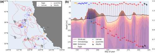
Each individual is moved around passively by the daily three-dimensional flow field provided by the hindcast simulation (Section 2.2; Figure 1a). In addition, pteropods undertake diurnal vertical migrations (DVM) with a size-specific velocity and within a depth range that increases with size from a few tens of meters in the juvenile stage to about 200 m in the case of adults (Figure 1b). This DVM is the main process through which pteropods are exposed to low and potentially very damaging Ω conditions at depth (Bednaršek & Ohman, 2015), where adults are bound to be more exposed than eggs or larvae owing to the progressively deeper migrations and given the strong decreases of Ω with depth. The current-driven drift and vertical swimming are calculated at a time-step of one hour, where the flow fields and environmental variables are interpolated from the current and next day in the hindcast simulation.
-
Shell growth: The shell growth is calculated from (i) the potential amount of CaCO3 an individual can produce given their current size and environmental conditions experienced in the absence of low Ω conditions, (ii) the accumulated damage from previous days, and (iii) the damage to the shell as a function of the experienced Ω (Hofmann Elizondo & Vogt, 2022). The exposure to Ω conditions below 1.5 can impede the growth of individuals through shell repair or shell mass loss once the protoconch has been developed. Following Bednaršek, Tarling, et al. (2014), the growth is reduced by the factor ν, which is a function of Ω and the fraction of the day (τ) a pteropod encounters low Ω conditions,
(1)
-
Mortality: Low Ω conditions and elevated temperatures tend to increase the daily mortality rate of an individual. Concretely, we adopt and modify the mortality function proposed by (Bednaršek et al., 2022), which increases the mortality rate as a function of Ω, temperature, and the exposure duration to :
(2)
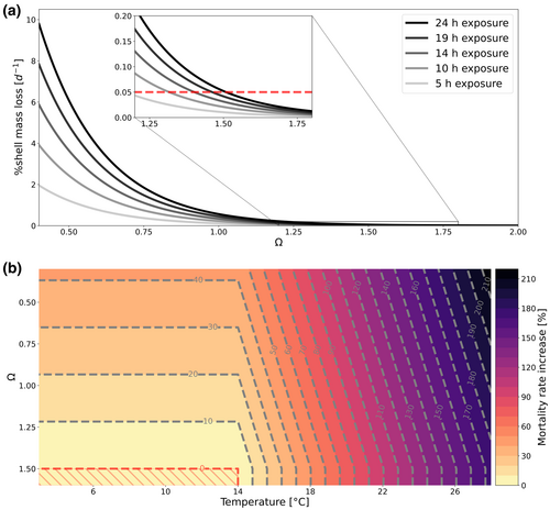
For temperatures less than the , the mortality rate increases up to 40% when Ω drops from 1.5 to 0.5 (see Figure 2b). For temperatures above this threshold, the mortality rate increases dramatically to more than 200%, when temperatures exceed 26°C and Ω approaches 0.5.
Given the key role of size in controlling the development of the pteropods, any growth reduction slows down the transition from one stage to the next one, where growth reductions delay the time until pteropods reach maturity, and increases in mortality rate may limit the number of individuals who reach the reproduction stage.
We also introduced flexible boundaries for the DVM and variable migration onset to the model to mirror the natural variability in pteropods' swimming behavior (Section A.4; Bednaršek & Ohman, 2015; Bianchi & Mislan, 2015). Additionally, a reseeding strategy was implemented to maintain pteropod populations within the CalCS (Section A.7). Finally, improvements to the mortality and shell growth functions were made by incorporating temperature effects on mortality (Bednaršek et al., 2022) and adjusting growth rates to include an upper thermal limit, aligning with empirical data and the observed thermal tolerance of L. helicina in the CalCS for a more realistic growth representation (see Section A.6).
2.2 Ocean biogeochemistry and circulation model
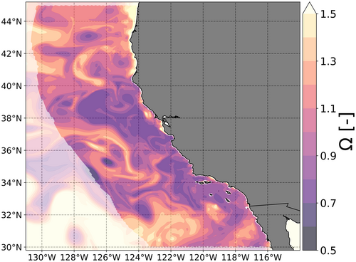
We use the results of a high-resolution hindcast simulation of the Northeast Pacific by Desmet et al. (2022) to provide the biogeochemical-physical forcing hazard associated with OA to the spIBM over the period 1984–2019. The model is based on the UCLA-ETHZ version of the regional oceanic modelling system (ROMS; Frischknecht et al., 2018; Marchesiello et al., 2002; Shchepetkin & McWilliams, 2005), coupled to the biological element cycling model (BEC; Frischknecht et al., 2017; Moore et al., 2013). Concretely, we use the daily three-dimensional fields of temperature, saturation state regarding the CaCO3 mineral aragonite, chlorophyll-a concentration, oxygen concentration, and the horizontal and vertical current velocities as input parameters for our spIBM in the central and southern part of the CalCS (between 30° N–45° N and 116° W–131° W within 500 km from the coast; Figure 3; Checkley & Barth, 2009). Other inputs include time, location, maximum depth, and land/water index for each grid cell. The ROMS-BEC model uses a telescopic grid with its center at the US West Coast (Frischknecht et al., 2018; Marchesiello et al., 2002) with a horizontal resolution of around 4 km in the CalCS and decreasing to around 60 km in the southwest Pacific, and 64 terrain-following vertical coordinates (Desmet et al., 2022). With this setup, the upwelling conditions, and basin-wide and local processes, for example, eddies that transport upwelled corrosive waters off the US West Coast, are properly simulated along the coastal region (Desmet et al., 2022; Frischknecht et al., 2015, 2017). Ω was calculated offline using the MOCSY 2.0 routine (Dickson et al., 2007; Orr & Epitalon, 2015) from daily model output for temperature, salinity, total alkalinity, silicate concentration, dissolved inorganic carbon, and total dissolved inorganic phosphorus.
The model successfully captures the observed variability and observed long-term changes in Ω (Desmet et al., 2022, 2023). However, in comparison to observational estimates of the gridded GLODAP version 2 Ω climatology (Lauvset et al., 2016), the model simulates a 26 m shallower median isoline and underestimates the median Ω in the simulation region by at most with an interquartile range of 0.3 (Figure B.1). Desmet et al. (2022) found similar deviations of the modelled Ω with those observed during the North American Carbon Program West Coast Cruise (Feely et al., 2008), which suggests a good representation of Ω in the CalCS. This underestimation in Ω results in a negligible increase in shell mass loss (; Section B.2) and can result in an absolute increase of the mortality rate by up to .
We use results from two ROMS-BEC simulations with the same model setup and forcing, covering the same period but forced with different atmospheric CO2 (Desmet et al., 2022, 2023). The first one is the standard hindcast simulation, where atmospheric CO2 is increasing as observed, and the lateral boundary conditions of dissolved inorganic carbon concentration in the Southern Ocean are increasing as well. In the second simulation, atmospheric CO2 and the lateral boundary conditions are held constant at about the 1979 levels, achieved by linearly detrending the respective time series. The difference between the two simulations reflects the long-term carbon emissions and ocean uptake since 1979.
2.3 Simulations with spIBM
We run the spIBM in the CalCS region (Section 2.2) from January 1 to December 31 for each year in the hindcast period (1984–2019). Individuals that drift outside of the simulation region are relocated within the CalCS using our reseeding strategy (Section A.7).
We start each year with the same initial population to ensure that changes in the simulated pteropods emerge only from the environmental conditions of the year of interest, and are not a legacy of previous years (cf. Dorman et al., 2011; Dorman, Sydeman, Bograd, & Powell, 2015; Dorman, Sydeman, García-Reyes, et al., 2015). As described in detail by Hofmann Elizondo and Vogt (2022), the life-stage composition of the starting pteropod population was obtained from a model spin-up with 5′000 days starting with a population of 1′500 eggs of the spring generation under idealized food availability and temperature, and without damaging conditions. This results in a population consisting primarily of juveniles, consistent with observations in the temperate region in winter (Dadon & de Cidre, 1992; Hsiao, 1939; Newman & Corey, 1984; Wang et al., 2017). The initial population is then randomly distributed in the CalCS, where positions near the coast have a higher probability of being chosen (see Section A.7). The spIBM is then run for 5 days in order to create the final initial conditions in terms of population size and life-stage composition.
We assess the impact of damaging conditions on individual pteropods by comparing their responses in the modeled scenarios to a hypothetical “Null” scenario, where no damage occurs (-scenario, Table 1), that is, where Ω is set to 1.5 for all locations and times with . This approach, allows pteropods to have the same trajectories across scenarios and model runs during simulations. In addition, the response to damaging conditions experienced are tracked for each individual pteropod in terms of size, accumulated damage, undersaturation experienced, and time of death for both scenarios.
| Scenario | Abbreviation | Modes of variability | Description |
|---|---|---|---|
| Full simulation | NTE | Natural variability, long-term trend, extreme events | Pteropods are affected by all components that result in damaging conditions |
| Extreme events set to | NT | Natural variability, long-term trend | Pteropods are affected by all components except extreme events |
| Constant CO2 without extremes | N | Natural variability | Pteropods are affected by the natural variability only |
| everywhere | None | Pteropods are not affected by damaging conditions |
2.4 Attribution
In addition to the “Null” () scenario, we define three additional scenarios to attribute the effects of damaging conditions to different modes of variability, such as (i) natural variability (denoted by N), (ii) long-term trend (denoted by T), and (iii) extreme events (denoted by E). These modes are defined as follows (see also Figure 4):
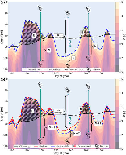
Natural variability (N): Naturally occurring damaging conditions, for example, at depth, that pteropods can experience in the CalCS with a baseline in the year 1979 (e.g., during DVM; Figure 1b).
Long-term trend (T): Increase in damaging conditions due to the long-term increase in carbon uptake by the ocean since 1979, and resulting OA. Most relevant is the shoaling trend of the isosurface.
Extreme events (E): Shorter term extreme events of damaging conditions, that is, areas where in the daily ROMS-BEC simulation, and in the daily climatology from the hindcast simulation (1984–2019).
This extreme event definition ensures that they only occur in places and days that are not expected to have based on the daily climatology. This definition differs from the often used relative threshold approach (see discussion in Gruber et al., 2021), for example, where an extreme only occurs if both pH and Ω fall below the 1st percentile of their local daily distribution in the period between 1984 and 2019 (Desmet et al., 2022). By adding the requirement of not being expected to occur based on the climatology, we have sharpened our definition of extremes and made their occurrence more rare.
The attribution of the damages to the different modes of variability is visualized in Figure 4, where the different types of exposure are indicated in a time-depth Hovmoeller diagram. When the isoline shoals above its climatological depth, the damage a pteropod accumulates while spending time in the cross-hatched watermass characterized by but being shallower than the climatological position of is attributed to Extremes (E) (Figure 4a). The damage accumulated below the climatological position of the isoline is attributed to natural processes (N). If we now include trends, which tend to lead to a shoaling of the isoline, the attribution to extremes remains the same, while the damage that accumulates below the (actual) isoline and also below the climatological position of the isoline is attributed to natural variability (N) and trends (T). Thus, the impact of trends can only be determined by considering the difference between simulations.
Since the full (hindcast) simulation considers all modes of variability, it corresponds to the NTE scenario (Table 1). To separate the roles of N, T, and E, we simulate two additional scenarios (Table 1): (i) No extremes, that is, called the NT-scenario. It is derived from the NTE-scenario by setting Ω to 1.5 for all identified extreme events. (ii) Natural variability only, that is, the N scenario. It is based on the constant CO2 simulation (Section 2.2), and is generated by setting Ω to 1.5 for all identified extreme events.
From these four scenarios, we determine the total impacts (all), and attribute them to the three modes of variability extremes (E), trend (T), and natural variability (N) by comparing model runs with specific exposure scenarios as shown in Table 2. This attribution approach allows us to circumvent the effects of the Ω biases modelled mortality, since the mortality function is linear (Equation 2), and the attribution is based on the relative comparison between scenarios (Section B.2).
| Description | Equation |
|---|---|
| Total impacts | (all) = f (NTE-scenario) − f (-scenario) |
| Impacts due to extremes | (E) = f (NTE-scenario) − f (NT-scenario) |
| Impacts due to the long-term trend | (T) = f (NT-scenario) − f (N-scenario) |
| Impacts due to the natural variability | (N) = f (N-scenario) − f (-scenario) |
2.5 Analyses and response metrics
To characterize the response of shelled pteropods to the exposure to damaging conditions we quantify the exposure to damaging conditions, the resulting shell damage, increased mortality risk, actual mortality or longevity decrease, and the long-term effects such as the decrease in recruitment success, and attribute the total exposure and impacts using our attribution scheme mentioned above.
Mortality increase relative to the -scenario: This metric quantifies the increased daily risk of dying due to the environmental conditions experienced (cf. Bednaršek et al., 2022; Bednaršek, Klinger, et al., 2017), using the weighted mortality rate (Section A.5) as a function of the temperature and undersaturation experienced by a pteropod in the NTE-scenario ().
Unlike continuous metrics, the binary nature of the longevity response prevents the application of the attribution scheme, which assumes progressively worse responses from the -scenario to the NTE-scenario. Thus, we determine the highest where each pteropod first dies across the NTE-, NT-, and N-scenarios (), and the attribution of the longevity decrease is calculated based on the contribution of each component to reach (see example in Section B.1).
2.5.1 Amplification of damaging conditions
2.5.2 Characteristics of damaging conditions
We quantify how the properties of individual exposure events, that is, intensity, duration, severity, recurrence, heterogeneity, and abruptness (Table 3), influence the modelled responses. Here, events are defined as the continuous number of days in which an individual experienced at least 1 hour of damaging conditions. These six properties were chosen, since they likely shape the response of marine organisms to extreme events (Gruber et al., 2021).
| Metric | Description | Unit |
|---|---|---|
| Intensity | Average decrease in Ω from Ω0 during an event. | |
| Duration | Cumulative duration of exposure to damaging conditions. | |
| Severity | Product of the intensity and duration of an event. | |
| Recurrence | Average time in which pteropods experience damaging conditions across their trajectory. | |
| Heterogeneity | Variance in intensity during an event. | |
| Abruptness | Speed at which the maximum intensity was reached during an event. |
These properties are specific to individuals that complete a full life-cycle in the model (spring generation; Section 2.1) and encounter damaging conditions. To determine the importance of each property as a predictor of the model's responses, we use mutual information (MI) (Cover & Thomas, 2005; Kinney & Atwal, 2014; Shannon, 1948). MI quantifies how much knowing one variable reduces uncertainty about another, essentially measuring the predictive strength of a property regarding the target variable. The value of MI indicates the relationship's strength, assessed in the context of the set of properties being tested.
2.5.3 Response to damaging conditions along the trajectory of the modelled pteropods
We compared our model result to a field study that examined pteropod shell damage as a function of decreasing Ω levels (Bednaršek, Feely, et al., 2014, see Figure B.2). We characterized the damaging conditions and CaCO3 changes in modelled pteropods that have reached at least the juvenile stage on the same day during the sampling year as in the field study. Additionally, we explored the link between prior exposure to damaging conditions along the simulated trajectories and the total CaCO3 loss observed during sampling.
3 RESULTS
3.1 Exposure to damaging conditions
Owing to the near continuous presence of waters with at depth, the modelled pteropods are exposed year-round to damaging conditions in the CalCS. At the same time, the upper waters are typically characterized by (Figure 5), such that the extent and depth to which the pteropods migrate vertically is the most important determinant for pteropod exposure (Figure 5). During the day, older and larger pteropods swim deeper during their DVM, and thus experience more damaging conditions compared to younger and smaller ones (Day in Figure 5). However, at night, pteropods are generally located near the surface to feed, where (Night in Figure 5).
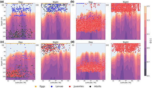
Averaged across all life-stages of the spring-generation, that is, those that can go through a full life-cycle in our model setup, a pteropod in the CalCS encounters damaging conditions during 36% of days of its lifespan. However, given the life-stage-dependent depth of the DVM, this fraction increases from 2% during the egg stage to 21%, 89%, and 99% during the larval, juvenile, and adult stage, respectively. Furthermore, for mature pteropods with an average lifespan of 184 days, this progressive increase in exposure throughout their life results in 131 days of experiencing damaging conditions, illustrating the challenging conditions that pteropods experience in the CalCS.
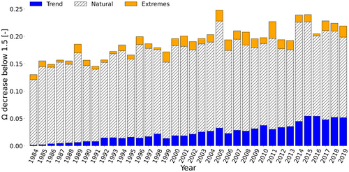
When exposed to such damaging conditions, the mean (±standard deviation) intensity of the exposure amounts to about over the analysis period (1984 through 2019; Figure 6). This implies an average Ω of . Over the course of the simulation, the intensity of damaging conditions increases from 0.13 (i.e., Ω 1.37) in 1984 to 0.22 (i.e., Ω 1.28) in 2019, and ranges between 0.13 (1984) and 0.25 (2005). While most of the intensity of damaging conditions experienced by pteropods is caused by natural variability (; mean ± standard deviation), the long-term trend and extremes drive the overall increase across the hindcast period (; Table B.1), as they amplify the intensity of the naturally occurring damaging conditions by 9% in 1984, and 49% in 2019 (Figure B.3), where 60% and 40% of this amplification is caused by the long-term trend and extreme events, respectively (Figure B.4).
3.2 Responses of pteropod populations to damaging conditions and its attribution
The average shell CaCO3 loss in all modelled individuals increases from 3% in 1984 to 7% in 2019, and ranges between 3% (1984) and 8% (2014) (Figure 7a). Averaged across the hindcast period, the natural variability in damaging conditions, the long-term trend, and extreme events are responsible for , , and of the shell CaCO3 loss, respectively. The CaCO3 loss due to the long-term trend and extremes increases across the hindcast period (; Table B.1). On average, they amplify the natural shell CaCO3 loss by 31% and 10%, respectively (Figure B.5A). Relative to natural variability, the long-term trend together with the extreme events increase the shell CaCO3 loss by at least 7% in 1984 and at most 102% in 2019 across the hindcast period (Figure B.5A).
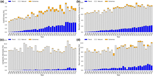
In all modelled individuals, the average increase in mortality probability caused by exposure to damaging conditions increases from 6% in 1984 to 9% in 2019, ranging between 6% (1992) and 10% (2011; Figure 7b). Averaged across the hindcast period, the natural variability component is responsible for of the increase in mortality probability, followed by the long-term trend () and extremes (). The mortality due to the natural exposure to damaging conditions during DVM has remained approximately constant since 1984 (; Table B.1). The long-term trend and extremes amplify the mortality caused by the natural variability component on average by 15% and 3%, respectively (Figure B.5B) where the mortality associated with extreme events and the long-term trend shows an increasing trend (from 4% in 1984 to 40% in 2019 relative to the natural variability; Figure B.5B).
The total longevity of the individuals did not change significantly during the simulation period (; Table B.1), despite the increasing trend in the decrease in longevity caused by the long-term trend and extreme events (; Table B.1). Thus, the difference between 1984 and 2019 is lower than the interannual variability, where the decrease in longevity relative to a scenario without damaging conditions amounts to 26% in 1984, increases to 30% in 2019, and ranges between 23% (2006) and 39% (2015; Figure 7c). In absolute number of days, this means that longevity is 30 days shorter across the hindcast period (see Figure B.7) where the natural variability of damaging conditions is responsible for of the decrease in longevity. The long-term trend () and extremes () play a minor role in the longevity reduction (Figure 7c).
The exposure to damaging conditions increases the fraction of individuals who die before spawning eggs by 8% in 1984 (Figure 7d). This fraction increases by 12% in 2019, and ranges between 7% (1992) and 13% (2013). The exposure to the natural variability, long-term trend, and extreme event components in damaging conditions are responsible for , , and of the decrease in recruitment, respectively. The decrease in recruitment due to the natural and long-term components of exposure shows an increasing trend (; Table B.1). The long-term trend and extreme events reduce the modelled recruitment by 3% in 1984 and by 25% in 2019 (Figure B.5D), where, the long-term trend and extreme events amplify the recruitment decrease due to the natural component on average by 13%, and 4%, respectively (Figure B.5D).
In general, the magnitudes of the four response metrics increase from 1984 toward 2019, where the modelled response is mostly caused by the natural variability of damaging conditions (>74%; Figure 7). On average, <20% of the modelled responses are caused by the long-term trend and <7% by extreme events. However, the long-term trend and extreme events increase the magnitude of the response in time. Averaged across the hindcast period, the long-term trend is responsible for the majority (>69%; Figure B.6) of the increase in response metrics (except the decrease in longevity). Key differences are seen between the observed patterns for the damaging condition and the modelled responses for the decrease in longevity and recruitment success. The former does not show an increasing trend across the hindcast period, and for the latter, the increase across the hindcast period is caused by the increasing trend in natural variability and the long-term trend, instead of the long-term trend and extreme events (Table B.1).
3.3 Characteristics of damaging conditions experienced
The exposure to intense and longer events of damaging conditions (Section 2.5.2 and Table 3) generally results in a higher CaCO3 loss, with low/high variability in CaCO3 loss at low/high intensities and short/long durations. The mean CaCO3 loss during an event increases from nearly 0% to 9% ± 9% with increasing intensity (Figure 8a), and it increases from 1 ± 1% (<10 days) to 16% ± 5% (>80 days) with increasing exposure duration (Figure 8b). The severity also shows an increasing pattern of CaCO3 loss as a function of damaging condition severity (Figure 8c). However, the uncertainty in CaCO3 remains stable across event severity; as reflected by the higher mutual information score (see Section 2.5.2; MI = 1.40) where the mean CaCO3 loss increases from 1 ± 1% at low severities (<5 days) to 24%±3% at high severities (>50 days).
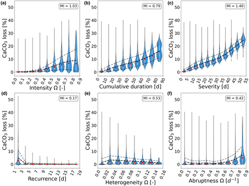
As shown by the mutual information scores, the recurrence (MI = 0.17), heterogeneity (MI = 0.53), and abruptness (MI = 0.42) of damaging conditions are poor predictors for the CaCO3 loss. However, we find that the mean CaCO3 loss decreases from 5% ± 6% for continuous events (less than every 3 days) to <1% as a function of increasing recurrence (≥3 days; Figure 8). In terms of heterogeneity, the mean CaCO3 loss remains relatively low and stable between 1%±1% and 3±3% as a function of the increasing heterogeneity. Finally, the mean CaCO3 loss remains relatively low and stable (between 1% and 2%) at low damaging event abruptness (<0.7 days−1) and increases to 7%±7% for events with the highest abruptness (>0.8 days−1; Figure 8).
Based on the mutual information scores (MI), the severity of damaging conditions (MI = 1.39) is best suited to explain the modelled CaCO3 loss among all the tested properties (Figure 8). Furthermore, the continuous exposure to damaging conditions (<3 d) and damaging events of high abruptness (>0.8 days−1) result in a high CaCO3 loss. Finally, changes in intensity across the event (heterogeneity) have a relatively low effect on the modelled response (MI = 0.53).
3.4 Dissolution across pteropod life-time
In general, an average individual that reaches maturity experiences damaging conditions during ~71% (131 days out of 184 days) of its life (Section 3.1). Thus, by only looking at individuals that reach later life-stages, we characterize the progression of exposure and responses along the life-history of pteropods. Due to the life-stage-dependent depth of their DVM (see Figure 5) shelled pteropods experience on average damaging conditions from the age of 43 ± 11 days onwards. Individuals encounter damaging conditions nearly every day and on average during 98% of the days of their juvenile and adult life-stage (cf. Figure B.8F). Throughout the life-history of the pteropod, the intensity of the damaging conditions experienced can vary between 0 and 0.93 (i.e., Ω 1.5 and 0.57, respectively), with an average intensity of (Ω 0.97 ± 0.20) between all individuals. Similarly, the duration of the exposure varies between 0 and 24 h with an average duration of exposure of 8 ± 6 h (Figure B.8E).
The near daily exposure to damaging conditions results in the accumulation of shell CaCO3 loss throughout the life-time of the modelled pteropods (Figure 9b), which amounts on average to 11% ± 10%, ranging between 0% (in the early stages of life) and 50%. Along the trajectory, the CaCO3 loss generally increases with an average daily CaCO3 loss of (Figure 10).
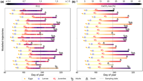
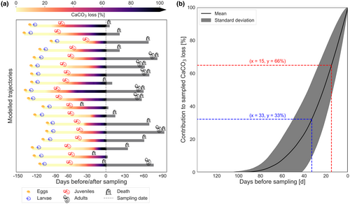
Therefore, modelled pteropods experience damaging conditions almost daily after reaching the juvenile stage and experience a Ω of 0.97 for approximately 8 h each day (Figure 9). This means that the accumulation of CaCO3 loss begins with the juvenile stage and increases at an average rate of As such, the modelled pteropods showed on average one-third of the accumulated damage 33 days before the sampling period began (Figure 10), demonstrating the importance of cumulative dissolution developing over time where the magnitude of damaging conditions and a prolonged exposure duration may lead to severe shell dissolution.
4 DISCUSSION
4.1 Intensity of the damaging conditions experienced by pteropod populations
In Eastern Boundary Upwelling Systems such as the CalCS, organisms regularly experience damaging conditions due to naturally low Ω conditions (Hauri, Gruber, McDonnell, & Vogt, 2013; Joint et al., 2010). In particular, shelled pteropods experience such conditions most regularly at depth (Bednaršek & Ohman, 2015), where they seek refuge from visual predation during the day (Hays, 2003; Zaret & Suffern, 1976). In the CalCS, we find that this DVM accounts for the majority of exposure to damaging conditions. However, even earlier life stages with a more limited extent of vertical migration are occasionally exposed to such damaging conditions, since upwelling events can cause Ω to reach values below 1.5 in the upper 60 m of the water column near the coast of the CalCS (Feely et al., 2008, 2009, 2016, 2018; Gruber et al., 2012; Hauri et al., 2009; Leinweber & Gruber, 2013; Turi et al., 2016). Furthermore, the combination of the long-term trend and extreme events has amplified naturally occurring damaging conditions from 9% in 1984 to ~50% in 2019 (Figure B.3), with the trend and extremes accounting for ~60% and ~40% of this overall increase, respectively (Figure B.4). This is in line with predicted increases in the total water volume of damaging conditions in the CalCS due to the long-term trend (Gruber et al., 2012), which increases the frequency of occurrence of undersaturation throughout the year in the CalCS (Harris et al., 2013; Hauri, Gruber, McDonnell, & Vogt, 2013; Hauri, Gruber, Vogt, et al., 2013).
Compared to previous studies, where the long-term trend is responsible for most (86% in 2011 compared to the preindustrial period) of the increase in experienced damaging conditions (see Table 1 in Bednaršek, Feely, et al., 2014), we find a greater contribution from the natural variability in experienced damaging conditions (82% across the hindcast period; Figure 6) and across all response metrics (e.g., 74% for CaCO3 loss; Figure 7a). The higher contribution from natural variability is explained by the fact that our study defines natural variability relative to 1979 (Section 2.2), whereas the baseline in Bednaršek, Feely, et al. (2014) is the preindustrial era. Accordingly, shifting our baseline to the preindustrial era would reduce the relative contribution of natural variability and increase that of the long-term trend and extreme events.
4.2 Attribution of responses of pteropod populations to damaging conditions
In the CalCS, where low Ω conditions have occurred since the preindustrial era (Gruber et al., 2012; Harris et al., 2013; Hauri, Gruber, McDonnell, & Vogt, 2013), migratory shelled pteropods are likely to have encountered such damaging conditions for centuries. This makes them a good indicator for changes in damaging conditions over time (Bednaršek et al., 2016; Bednaršek, Klinger, et al., 2017; Manno et al., 2017; Mekkes et al., 2021). Furthermore, the long-term trend of OA and extreme events increase the magnitude, duration, and volume of damaging conditions in the CalCS (Burger et al., 2020; Desmet et al., 2023; Gruber et al., 2012, 2021), which—as shown in this study—means that migratory shelled pteropods experience more intense, prolonged, and frequent damaging conditions. Therefore, it follows that monitoring programs must take into account all factors determining the overall exposure to damaging conditions when evaluating the impacts on pteropods (cf. Bednaršek, Klinger, et al., 2017). Our model now provides a clear separation between the effects of natural variability, long-term OA trends, and extreme events. As such, it establishes a baseline specifically for the responses to natural recurring damaging conditions, which is essential for isolating the impact of OA in a region.
However, in future OA studies, it is necessary to consider the interplay of pteropod DVM and life-history with naturally occurring damaging conditions, the long-term OA trend, and extreme events (Figure 5; Bednaršek, Feely, et al., 2017). This becomes evident by comparing the potential exposure across the entire upper 250 m of the water column in the CalCS (Figure B.9 with the realized exposure Figure 6), where, on average, the intensity of the realized exposure is 58% lower than the potential exposure. This water column average approach, while easier to measure in the field, tends to overestimate the intensity of damaging conditions experienced by migratory pteropods (Bednaršek & Ohman, 2015), and neglects other key exposure properties (e.g., exposure duration; Bednaršek et al., 2021; Gruber et al., 2021). Thus, by associating the observed damage with the higher potential exposure rather than the realized exposure, the sensitivity of pteropods to damaging conditions can be consistently underestimated. For example, removing the duration of exposure from the model can double the increase in the probability of mortality from around 10% (Figure 7b) to ~20% in 2011 (Figure B.10).
Another key aspect that determines the simulated responses is the life-history of the individuals and their prior exposure to damaging conditions (Figure 9). Recent studies suggest that life-history and prior exposure; particularly during early life-stages; likely determine the individual's response to damaging conditions later in life, as well as changes in population demographics (Bednaršek et al., 2016; Bednaršek, Feely, et al., 2017). Furthermore, damage has been observed to accumulate over an individual's life-time, as evidenced by differences in dissolution marks on the shell between studies conducted in different times in CalCS (Mekkes et al., 2021). However, most current OA impact studies do not consider the trajectories of observed individuals (but see Bednaršek, Feely, et al., 2017), as this cannot easily be done with an Eulerian framework, which links individual responses to local environmental conditions (Bednaršek et al., 2022; Bednaršek, Feely, et al., 2014; Mekkes et al., 2021). Consequently, our model characterizes the cumulative effects of recurrent exposure to damaging conditions and links them to the individual's life-history rather than the environmental conditions during sampling (Figure 10). As such, 33 days before sampling, our model predicts that the pteropods had already incurred a substantial amount (one-third) of the observed CaCO3 loss on average (Figure 10).
This individual perspective, combined with the overall response attribution and change over time (Figure 7a), suggests that the majority of the accumulated damage is primarily caused by natural variability. Furthermore, our analyses show that the first 43 days after spawning do not contribute to dissolution. Thus, it is important to analyze the entire life-history to avoid underestimating the dissolution. Examining the average spring individual across the hindcast simulation (Figure B.11), we observe an overall increase in CaCO3 loss from 1984 to 2019, with natural variability accounting for most of the damage. However, the contribution of natural variability to the CaCO3 loss decreases over the hindcast period, while that of the long-term trend increases. Finally, we observe that extreme events contribute to CaCO3 loss, particularly during early life-stages when individuals have a relatively shallow DVM and spend more time near the interface between damaging and non-damaging conditions (Figure 4).
Accurate characterization of the responses of pteropods to damaging conditions along their trajectories is crucial to assess potential changes in population dynamics, such as mortality and recruitment success (Sinclair, 1997). Although pteropods are sensitive to changes in Ω (Bednaršek et al., 2016; Bednaršek, Klinger, et al., 2017; Bednaršek & Ohman, 2015), there is no clear indication of a decrease in shelled pteropod abundance from measured abundance in the CalCS (Doo et al., 2020; Ohman et al., 2009). Here, we confirm these findings based on the simulated pteropod longevity (Figure 7c) and recruitment success (Figure B.12A). Although mortality probability has been increasing since 1984, the longevity of pteropods has not decreased significantly during the same period (Table B.1), probably because the naturally high mortality for the species (Bednaršek et al., 2012) represents the driving process. This suggests that the Ω decrease due to the long-term OA trend and extremes has not yet led to a significant decline in simulated longevity, with natural variability remaining the driving factor in the reduction of longevity. In terms of impact, we did not observe a significant decrease in recruitment success over the hindcast simulation (Section B.12; Figure B.12A). Thus, our results are consistent with the findings of Ohman et al. (2009) that despite the sensitivity of pteropods to changes in ocean chemistry, the long-term OA trend and the extreme events have not yet caused a measurable change in the abundance of pteropods (cf. Doo et al., 2020; Mackas & Galbraith, 2012).
Overall, our model aligns well with previous observations and predictions about shelled pteropod exposure to damaging conditions, enabling us to disentangle the influence of environmental drivers across different scales. The attribution framework developed herein can be applied to other species and regions and, together with the model, can be used to investigate responses of pteropod populations across different time-scales (acidification increase/decrease during summer/winter; Kwiatkowski & Orr, 2018). However, the spIBM is specifically calibrated to the CalCS and primarily based on L. helicina (Section 2.1; Hofmann Elizondo & Vogt, 2022). Therefore, the spIBM functions (Section 2.1) need to be adjusted for the respective functional group and calibrated to the region of interest (Hofmann Elizondo & Vogt, 2022).
4.3 Caveats and limitations
Multiple sources of biases and limitations need to be considered. A first source of potential bias in our study stems from the hindcast simulation that provides the time-varying environmental conditions that drive the spIBM. While the hindcast simulation reproduces the large-scale climatological state of the North Pacific Ocean and coastal upwelling strength (cf. Desmet et al., 2022), it underestimates Ω by around (Section B.2). This implies that pteropods tend to encounter damaging conditions at shallower depths and that they are exposed to higher intensities of damaging conditions at depth. However, since we calculate the response and attribution relative to a reference scenario with the same bias (Table 1) and the resulting biases in shell CaCO3 loss are negligible, and those in mortality are linear, such time-invariant biases have a limited impact on our results (Section B.2). Further, this approach allows us to focus on changes in environmental conditions rather than the underestimated values on individual days. Thus, with our model we can reproduce observed patterns that accurately capture the relative differences, but may not align with the exact location and absolute magnitude of the response (e.g., Figure B.14).
A second source of uncertainty arises from our definition of the three components of the damaging conditions in the CalCS (Section 2.4). Throughout the analysis, the natural variability drives the modelled responses, while the long-term OA trend and extremes increase the number of encounters with damaging conditions and their intensity. The dominance of the natural component may result from the way we define natural variability, long-term trend, and extreme events. Specifically, the long-term trend is based on the first year of the hindcast simulation (1979; (Desmet et al., 2022)) rather than the preindustrial era (Section 2.2), and the extreme events are determined based on the mean of the hindcast period. Nevertheless, our approach and attribution align with recent and ongoing time-series monitoring programs (Ohman & Venrick, 2003), and recurrent cruises (West Coast Ocean Acidification cruises; Bednaršek et al., 2022; Bednaršek, Feely, et al., 2014; Mekkes et al., 2021), where these programs use a baseline or reference period determined by the time of the first measurements (1951 for the California Cooperative Oceanic Fisheries Investigations program; Ohman, 2021; Ohman & Venrick, 2003).
An additional uncertainty arises from our assumption that the modelled pteropods cannot adapt to the changing conditions since 1979, despite their adaptation potential and acclimatization capabilities (cf. Peijnenburg et al., 2020). Furthermore, the potential influx of individuals from other populations, or variations at small spatial scales, could potentially reduce the magnitude of the response to environmental changes (Choo et al., 2021). However, pteropods over large spatial scales; for example, the North Pacific; show very low genetic variability within a population (Bednaršek et al., 2021; Mekkes et al., 2021), demonstrating that adaptation processes might not occur at the rates to leverage increasing sensitivity. As such, the adaptive capabilities of pteropods to a changing environment are likely more relevant on longer time scales compared to the contemporary, rapid, and unprecedented environmental changes (cf. Peijnenburg et al., 2020). In addition, our approach aligns well with the finding that it is particularly the exposure of the early life-stages that have the most negative effects on pteropod population demographics Bednaršek et al. (Bednaršek et al., 2016; Bednaršek, Feely, et al., 2017).
5 CONCLUSION
This study identifies various temporal modes of environmental variability that define damaging conditions for shelled pteropods. Our simulations demonstrate that most pteropod responses are caused by naturally occurring exposure to damaging conditions at depth during DVM. However, long-term trends and extreme events have increasingly influenced pteropod responses since 1984, and are expected to continue doing so. Consequently, monitoring programs (Feely et al., 2016; Mackas & Galbraith, 2012; Ohman & Venrick, 2003) need to distinguish between damages caused by natural variations and those caused by long-term trends and extremes, thus establishing species- and region-specific baselines. IBMs and other Lagrangian models play a key role in linking observed responses with the life histories and trajectories of pteropods (e.g., Bednaršek, Feely, et al., 2017). Developing such detailed scenarios is critical to evaluate human influences on pteropod populations and distinguish them from natural variations, thus guiding decision makers to establish effective monitoring and management practices for the conservation of coastal ecosystems.
In this study, we focus on the response of shelled pteropods to variations in Ω, neglecting their exposure to a diverse set of other relevant environmental conditions throughout their trajectory (Figure 1b). To improve the accuracy and predictive potential of our IBM, it is necessary to incorporate other environmental factors, such as temperature and food availability, especially given that future environmental changes include warming and decreasing chlorophyll levels (Bednaršek et al., 2016, 2022; Le Grix et al., 2021). These factors, along with acidification, could exacerbate the negative impacts on shelled pteropods, increasing mortality, and affecting growth during periods of scarce food. Currently, our model simulates the temperature and food dependence of growth and mortality. The next step involves expanding the model to include simulations that integrate multiple environmental variables and analyzing pteropods reactions to individual and combined stressors (Burger et al., 2020; Frölicher et al., 2018; Gruber et al., 2021).
Finally, our model and attribution scheme offer the potential for studying other dominant pteropod species in regions like the Southern Ocean, where pteropods are crucial for the plankton community (Hunt et al., 2008), and undersaturation will increase in the near future (Orr et al., 2005). Additionally, this attribution scheme can be expanded to assess the impact of environmental stressors on different organisms, such as krill (Dorman, Sydeman, Bograd, & Powell, 2015) or copepods (Miller et al., 1998). By integrating historical fisheries yield data, alterations in modeled populations due to environmental stressors can be directly linked with changes in energy transfer across trophic levels (Capuzzo et al., 2017; Field et al., 2006; Lindley et al., 2009; Ware, 2005), providing policymakers with a direct link between environmental stressors, economic implications, and food security for various emission scenarios (van Oldenborgh et al., 2021).
AUTHOR CONTRIBUTIONS
Urs Hofmann Elizondo: Conceptualization; data curation; formal analysis; investigation; methodology; software; validation; visualization; writing – original draft; writing – review and editing. Meike Vogt: Conceptualization; funding acquisition; methodology; project administration; supervision; visualization; writing – review and editing. Nina Bednaršek: Methodology; writing – review and editing. Matthias Münnich: Conceptualization; funding acquisition; methodology; project administration; supervision; visualization; writing – review and editing. Nicolas Gruber: Conceptualization; funding acquisition; methodology; project administration; resources; supervision; visualization; writing – review and editing.
ACKNOWLEDGEMENTS
We thank Flora Desmet, Eike Köhn, and the Environmental Physics group for analytical and visualization advice. Open access funding provided by Eidgenossische Technische Hochschule Zurich.
FUNDING INFORMATION
This research was supported by ETH Zürich under grant 175,787—‘X-EBUS: Extreme Ocean Weather Events and their Role for Ocean Biogeochemistry and Ecosystems in Eastern Boundary Upwelling Systems’ (SNF).
CONFLICT OF INTEREST STATEMENT
The authors declare that there is no conflict of interest.
Open Research
DATA AVAILABILITY STATEMENT
The code used in this manuscript can be obtained from https://github.com/ursho2552/Multiscenario_Shelled_Pteropod_IBM and Zenodo at https://doi.org/10.5281/zenodo.11096564. All analyses and figures were created using the software package Python. The input to the IBM stemming from the high-resolution model simulation of Desmet et al., as well as the IBM output are available on Dryad at https://doi.org/10.5061/dryad.wh70rxww9. All further analysis scripts may be obtained upon request from the corresponding author ([email protected]).


