Do dynamic global vegetation models capture the seasonality of carbon fluxes in the Amazon basin? A data-model intercomparison
Abstract
To predict forest response to long-term climate change with high confidence requires that dynamic global vegetation models (DGVMs) be successfully tested against ecosystem response to short-term variations in environmental drivers, including regular seasonal patterns. Here, we used an integrated dataset from four forests in the Brasil flux network, spanning a range of dry-season intensities and lengths, to determine how well four state-of-the-art models (IBIS, ED2, JULES, and CLM3.5) simulated the seasonality of carbon exchanges in Amazonian tropical forests. We found that most DGVMs poorly represented the annual cycle of gross primary productivity (GPP), of photosynthetic capacity (Pc), and of other fluxes and pools. Models simulated consistent dry-season declines in GPP in the equatorial Amazon (Manaus K34, Santarem K67, and Caxiuanã CAX); a contrast to observed GPP increases. Model simulated dry-season GPP reductions were driven by an external environmental factor, ‘soil water stress’ and consequently by a constant or decreasing photosynthetic infrastructure (Pc), while observed dry-season GPP resulted from a combination of internal biological (leaf-flush and abscission and increased Pc) and environmental (incoming radiation) causes. Moreover, we found models generally overestimated observed seasonal net ecosystem exchange (NEE) and respiration (Re) at equatorial locations. In contrast, a southern Amazon forest (Jarú RJA) exhibited dry-season declines in GPP and Re consistent with most DGVMs simulations. While water limitation was represented in models and the primary driver of seasonal photosynthesis in southern Amazonia, changes in internal biophysical processes, light-harvesting adaptations (e.g., variations in leaf area index (LAI) and increasing leaf-level assimilation rate related to leaf demography), and allocation lags between leaf and wood, dominated equatorial Amazon carbon flux dynamics and were deficient or absent from current model formulations. Correctly simulating flux seasonality at tropical forests requires a greater understanding and the incorporation of internal biophysical mechanisms in future model developments.
Introduction
Dynamic global vegetation models (DGVMs) are the most widely used and appropriate tool for predicting large-scale responses of vegetation to future climate scenarios. However, to forecast the future of Amazonia under climate change remains a challenge. The previous generation of DGVMs produced projections for Amazonia's ecosystems that diverged widely, with outcomes ranging from large-scale forest dieback to forest resilience (Betts et al., 2004; Friedlingstein et al., 2006; Baker et al., 2008). More recent DGVM simulations showed the large-scale die-off scenario to be unlikely (Cox et al., 2013), given (i) an improved model understanding of forest response to the negative effects of temperature previously overestimated and now constrained (Cox et al., 2013), and (ii) current models being forced with updated climate projections (temperature and precipitation) bounded by observations that no longer demonstrate drastic climate changes in response to rising CO2 in the tropics (Cox et al., 2013; Huntingford et al., 2013). Yet tropical forest response to climate change remains uncertain as models produce varying outcomes (Shao et al., 2013) even without die-off. Some cutting-edge DGVMs projected forest degradation due to future deforestation and increasing temperature, with catastrophic consequences for the global climate based on climate–carbon cycle feedbacks (Wang et al., 2013, 2014; Friend et al., 2014), while other DGVMs foresaw strong carbon sinks in these forests due to CO2 fertilization of photosynthesis (Rammig et al., 2010; Ahlström et al., 2012; Huntingford et al., 2013; Friend et al., 2014). Although the effects of temperature, water limitation, and CO2 fertilization mechanisms remain uncertain, all DGVMs continue to agree that Amazonian forests play an important role in regulating the global carbon and water cycle (Eltahir & Bras, 1994; Werth & Avissar, 2002; Wang et al., 2013, 2014; Ahlström et al., 2015).
Key to reducing uncertainty in DGVMs is their systematic evaluation against observational datasets. This exercise enables the identification of model deficiencies through comparison with observed patterns in ecosystem processes, as well as the mechanisms underpinning such processes (Baker et al., 2008; Christoffersen et al., 2014). Recent model-data evaluations in tropical forests have focused on the cascade of ecosystem responses to long-term droughts (Powell et al., 2013) and the definition of spatial patterns in productivity and biomass (Delbart et al., 2010; Castanho et al., 2013). However, one important context for model assessment in tropical forests is in the seasonality of ecosystem water and carbon exchange, as observational datasets reveal axes of variation in productivity, biomass and/or forest function across space (da Rocha et al., 2009; Restrepo-Coupe et al., 2013), and/or through time (Saleska et al., 2003; von Randow et al., 2004; Hutyra et al., 2007; Brando et al., 2010). The most consistent temporal variation in tropical forests is the seasonality of water, energy, and carbon exchange, as all tropical ecosystems are seasonal in terms of insolation and a majority experience recurrent changes in precipitation, temperature, and/or day length. Evaluation with respect to seasonality has typically focused on evapotranspiration (ET) (Shuttleworth, 1988; Werth & Avissar, 2002; Christoffersen et al., 2014) and on net carbon exchange (NEE) (Baker et al., 2008; von Randow et al., 2013; Melton et al., 2015). Where models compensated misrepresentations of gross primary productivity (GPP) in the NEE balance, by improving or adjusting the efflux term represented by heterotrophic (Melton et al., 2015) or ecosystem respiration (Baker et al., 2008) to available moisture among other strategies. Only recently have the seasonal dynamics of GPP drawn the attention of different groups (De Weirdt et al., 2012; Kim et al., 2012) and where Kim et al. (2012) demonstrated that a consequence of its incorrect derivation was to overestimate the vulnerability of tropical forests to climate extremes. Therefore, identifying discrepancies in observed vs. modeled seasonality in carbon flux even when seasonal amplitudes are not large, as can be the case for evergreen tropical forests (see LP Albert, N Restrepo-Coupe, MN Smith et al. (submitted) for cryptic phenology), can lead to important model developments with significant consequences to obtain better projections of the fate of tropical ecosystems under present and future climate scenarios.
Analysis of eddy covariance datasets has shown that in non-water-limited forests of Amazonia, the observed seasonality of GPP was not exclusively controlled by seasonal variations in light quantity (as has been demonstrated for ET) or water availability. Instead, GPP was driven by a combination of incoming radiation and phenological rhythms influencing leaf quantity (measured as leaf area index; LAI) and quality (leaf-level photosynthetic capacity as a function of time since leaf-flush) (Restrepo-Coupe et al., 2013; Wu et al., 2016). The lack of a direct correlation between GPP and climate suggests that ecosystem models that are missing sufficient detail of canopy leaf phenology will likely not capture seasonal productivity patterns. Accordingly, recent studies showed model simulations (ED2 and ORCHIDEE) to be deficient in terms of predicted seasonality in GPP and litter-fall, if missing leaf demography and turnover as in Kim et al. (2012) and in De Weirdt et al. (2012), respectively. Between the two studies, only two sites (eastern ‘K67’ and northeastern (‘CAX’) were represented, both of which experience very similar precipitation and light regimes. This further highlights the need for expanded evaluation of modeled seasonality of GPP across a range of sites spanning a broader range of climates and phenologies.
If the improved representation of the dynamics of leaves and other carbon pools translates into more accurate simulations of seasonal GPP and/or the long-term carbon budget (De Weirdt et al., 2012; Kim et al., 2012; Melton et al., 2015), then comparisons between observations and model-derived seasonality of carbon allocation could provide insight into the mechanistic response of vegetation to climate and strategies to incorporate them into DGVMs. For example, critically evaluating the seasonality of net primary production of leaves (NPPleaf) and wood (NPPwood) in tandem with photosynthesis will inform deficiencies in model allocation schemes and carbon pool residence times. Model net primary production (NPP) typically arises from the allocation of photosynthate to main organs, either as a constant fraction of GPP (Kucharik et al., 2006), or according to fixed allometric rules (Sitch et al., 2003). However, such a view of supply-limited growth has come into question recently (Würth et al., 2005; Fatichi et al., 2014). Thus, as water, temperature, and nutrients can all impact cell expansion, there may be a temporary imbalance between carbon used for tissue growth and maintenance respiration vs. carbon supplied by assimilation (photosynthesis) (Fatichi et al., 2014). Patterns in seasonality of GPP, NPPleaf, and NPPwood, therefore, potentially reveal the degree of coupling (or lack thereof) of these two carbon sinks (NPPwood and NPPleaf) with photosynthetic activity (GPP). Indeed, Doughty et al. (2014) used bottom-up estimates of the ecosystem carbon budget at a forest in southwest Amazonia and showed that components of NPP varied independently of photosynthetic supply, which they interpreted in terms of theories of optimal allocation patterns. While an alternative interpretation of such patterns could simply refer to biophysical limitations on growth, which vary seasonally (Fatichi et al., 2014), both studies suggest that modeling allocation as a function of GPP will likely fail to capture observed seasonality. Ground-based bottom-up estimates of primary productivity at a temporal resolution greater than a year (i.e., seasonal) are difficult if not impossible, principally because there is no accepted method for estimating whole-tree nonstructural carbon (NSC) and its variation with seasons (Würth et al., 2005; Richardson et al., 2015). We propose coupling colocated top-down eddy flux estimates of GPP with bottom-up NPP estimates (NPPwood, NPPleaf, and NPPlitter-fall) to circumvent this problem and to obtain a better informed view of the mechanisms (e.g., allocation schemes) models may incorporate or test against, to improve seasonal simulations of carbon fluxes and pools.
The focus of this study was to evaluate, for the first time, modeled seasonal cycles of different carbon pools and fluxes, including leaf area index (LAI), GPP, leaf-fall, leaf-flush, and wood production, with high-resolution eddy flux estimates of GPP and ground-based surveys. We centered our study on a comparison between forests located in the equatorial Amazon (radiation- and phenology-driven) to a southern forest (driven by water availability) and explored the different model strategies to incorporate and simulate physical and ecological drivers. Here, we assessed four state-of-the-art DGVMs in active development for use in coupled climate–carbon cycle simulations in terms of whether they could simultaneously determine patterns of growth and photosynthesis, thereby getting the ‘right answer for the right reason’. We conclude by proposing several approaches for improving model formulations and highlight the need for model-informed field campaigns and future experimental designs.
Materials and methods
Site descriptions
We analyzed data from the Brazil flux network for four tropical forests represented by the southern site of Reserva Jarú (RJA), and three central Amazonia forests (~3°S) from west to east: the Reserva Cuieiras near Manaus (K34), the Tapajós National forest, near Santarém (K67), and the Caxiuanã National forest near Belém (CAX) (Fig. 1). For detailed site information see previous works by Restrepo-Coupe et al. (2013), and de Goncalves et al. (2009); de Gonçalves et al. (2013) and individual site publications (Araújo et al., 2002; Carswell et al., 2002; Malhi et al., 2002; Saleska et al., 2003; Kruijt et al., 2004; von Randow et al., 2004; Hutyra et al., 2007; da Costa et al., 2010; Baker et al., 2013).

All study sites had mean annual precipitation (MAP) above 2000 mm yr−1 (Fig. S1 and Table 1), based on the 1998–2014 satellite-derived precipitation from the Tropical Rainfall Measuring Mission (TRMM 3B43-v7 at a resolution of 0.25 deg) (Huffman et al., 2007; NASA, 2014). See Fig. S10 for a comparison between observations and TRMM data. CAX and K34 had MAP over 2500 mm yr−1, 2572, and 2673 mm yr−1, respectively (Fig. S11). By contrast, at the southern forest of RJA and at the equatorial forest of K67 MAP was ~2030 mm yr−1. We defined the dry season as those periods where precipitation was less than ~100 mm month−1 (Sombroek, 2001; da Rocha et al., 2004; Restrepo-Coupe et al., 2013). The 100 mm month−1 threshold corresponds to ~90% of the observed annual maximum 16-day ET averaged across years (115 ± 12 mm month−1) and close to the mean seasonal ET (92 ± 1.5 mm month−1) at the four tropical forests here reported (Restrepo-Coupe et al., 2013). Based on the 16-year TRMM series, RJA had a 5-month dry-season length (DSL) comparable to two of the central Amazon sites of CAX and K67 (4–5 months); however, longer than at the equatorial Amazon K34 forest (1–2-months). RJA and K67 showed similar mean dry-season precipitation (46 mm month−1 at RJA and 64 mm month−1 at K67). However, the annual minimum averaged across the years 1998–2014 (MiAP) at RJA was 15 mm month−1 compared to a more benign dry season minimum of 36 mm month−1 at K67 (Figs. 1 and S11, and Table 1). Despite being located at a latitude further from the equator (10°S), incoming photosynthetic active radiation (PAR) at the southern forest of Jarú was less seasonal (lower amplitude) if compared to the central Amazon forests (latitude ~3°S) (Fig. 2). At RJA, the period of peak top of the atmosphere radiation (TOA) was synchronous with the wet season – when we expected higher reflectance by clouds to decrease the surface available PAR (Fig. 2). All equatorial sites sat on highly weathered deep clay soils (≥10 m), whereas RJA sat on a lower water storage capacity loamy sandy soil and a more shallow and variable profile, with depth to bedrock as shallow as 2–3 m (Hodnett et al., 1996; Christoffersen et al., 2014).
| Site | Latitude | Longitude | Mean annual precipitation MAP (mm yr−1) | Dry-season precipitation DSP (mm month−1) | Dry-season length DSL (months) | Annual minimum average precipitation MiAP (mm month−1) | |
|---|---|---|---|---|---|---|---|
| K34 | −2.61 | −60.21 | 2672.6 | 99.7 | 1a | 99.7 |
|
| CAX | −1.72 | −51.53 | 2571.8 | 78.8 | 4 | 59.5 | |
| K67 | −2.86 | −54.96 | 2037.8 | 63.7 | 4a | 36.2 | |
| RJA | −10.08 | −61.93 | 2019.3 | 46.2 | 5 | 14.6 |
- a 1+ month DSL if defined as rain<103 mm month−1. TRMM 1998–2014.

Eddy covariance methods
 (1)
(1)Starting with half-hourly CO2 flux data provided from each site's operator, we calculated net ecosystem exchange (NEE in μmol CO2 m−2 s−1), with fluxes to the atmosphere defined as positive. NEE was then filtered for low turbulence periods (u* thresh). For a detailed description of instrumentation, data processing, applied corrections, quality control procedures, and the effect of u* thresh on NEE calculations refer to Restrepo-Coupe et al. (2013). Gross ecosystem exchange (GEE) was derived from tower measurements of daytime NEE by subtracting estimates of ecosystem respiration (Re), which we derived from the nighttime NEE. We assumed daytime Re was the same as nighttime Re, as we did not observe a statistically significant within-month correlation between nighttime hourly NEE and nighttime Tair (Restrepo-Coupe et al., 2013). GEE is a negative value (GEE = NEE - Re) as generally NEE is negative in the daytime, and Re is positive (meteorological convention). We expressed ecosystem-scale photosynthesis or gross ecosystem productivity (GEP), as negative GEE and assumed negligible re-assimilation of metabolic respiration CO2 within the leaf and insignificant CO2 recirculation below the EC system (Stoy et al., 2006). For comparison with model output, we used GEP interchangeably with gross primary productivity (GPP).
We defined ecosystem photosynthetic capacity (Pc, gC m−2 day−1) as the 16-day GPP averaged over a fixed narrow range of reference climatic conditions following some of the modifications introduced by Wu et al. (2016) (e.g., including CI and Tair on its calculations) to Pc used in Restrepo-Coupe et al. (2013). For our analysis, Pc was estimated as the rate of carbon fixation under reference conditions defined by fixed narrow bins in: site specific daytime annual mean PAR ± 150 μmol m−2 s−1, VPD, Tair, and CI ± 1.5 standard deviation from their respective means (see Table S1). Thus, Pc, by definition, removed the effect of day-to-day changes in available light, diffuse/direct radiation, photoperiod, temperature, and atmospheric demand from photosynthesis. The Pc has been shown to be a robust representation of the emergent photosynthetic infrastructure of the whole forest canopy (Wu et al., 2016).
We looked at evapotranspiration (ET, mm day−1) calculated as the latent heat flux (LE, W m−2) measured at the tower multiplied by the latent heat of vaporization (λ, kJ kg−1). We developed a Type II linear model between surface incident short-wave radiation (SWdown, W m−2) and the dependent variable, ET.
From the standard suite of climatic variables available for periods between 1999 and 2006 measured at each EC tower, meteorological drivers for the models were generated. According to Rosolem et al. (2008), the selected periods represent the mean climatological condition and exclude anomalous climatic events (e.g., 2010 El Niño-Southern Oscillation (ENSO) or 2005 drought as experienced at the southern Amazon). Variables included the following: SWdown; air temperature (Tair, °K); near-surface specific humidity (Qair, g kg−1); rainfall (Precip, mm month−1); magnitude of near-surface wind (WS, m s−1); surface atmospheric pressure (Pa, hPa); surface incident long-wave radiation (LWdown, W m−2); and CO2 concentration (CO2 air) was fixed at 375 ppm (de Goncalves et al., 2009) (Fig. 2). Drivers were created for consecutive years where gaps were no greater than two months. All time series were subject to quality control (e.g., removal of outliers) and then filled using other tower measurements (e.g., from a temperature profile), nearby sites and/or the variable's mean monthly diurnal cycle (Stockli, 2007). We analyzed data for 2000–2005 for K34, 2002–2004 for K67, 2000–2002 for RJA, and 1999–2003 for CAX. We restricted flux and meteorological observations and the calculation of seasonality to the above-mentioned dates in order to match model drivers and output.
Hourly fluxes (GPP, NEE, Re, and ET) and meteorology were aggregated to 16-day time periods, assuming that at least 4 days were available with at least 21 h of observations each. Gaps were not filled further and mean annual cycles were then calculated.
Field measurements
Although field measurements can be translated into carbon storage values (e.g., wood carbon pool from DBH inventories via allometric equations), we focused on departures from a base level because they reflect the seasonality of allocation. The following vegetation infrastructure descriptors and carbon pools were included in the analysis:
 (2)
(2)Leaf litter-fall or net primary productivity allocated to litter-fall (NPPlitter-fall, gC m−2 day−1): values corresponded to monthly litter-bed measurements at Manaus, K34 (here presented for the first time), and to those reported by Rice et al. (2004) for K67 and by Fisher et al. (2007) for CAX.
 (3)
(3)where specific leaf area (SLA) values were set to 0.0140 for K67 and CAX (Domingues et al., 2005), 0.0164 m2 per gC for K34 (Carswell et al., 2002). The Amax was reduced to reach 40% of the mean value at the time when leaf-fall reached its maximum (2-month linear gradient). Maximum Amax was set to 8.66 gC m−2 day−1 at K67 (Domingues et al., 2005), and to 7.36 gC m−2 day−1 at K34 (Carswell et al., 2000) and CAX.
Wood net primary productivity (NPPwood) was based on stem wood increment measurements (diameter at breast height, DBH) as reported by Rice et al. (2004) at K67, Chambers et al. (2013) at K34, and da Costa et al. (2010) at CAX and on allometric equations as proposed by in Chambers et al. (2001). No data were available for RJA.
Dynamic global vegetation models (DGVMs)
We presented output from four state-of-the-art dynamic global vegetation models. All DGVMs were process based (e.g., photosynthesis, respiration, and evapotranspiration) and able to simulate the fluxes of carbon, water, and energy between the atmosphere and the land surface (see Tables S2 and S3). The model simulations were run as part of the Interactions between Climate, Forests, and Land Use in the Amazon Basin: Modeling and Mitigating Large Scale Savannization project (Powell et al., 2013;).
To standardize all physical parameters within the models so as to focus on agreements and discrepancies among the different biomass schemes, all four DGVMs used the same soil hydrology properties (including free drainage conditions), and soil physical parameters and depths. The spin-up protocol consisted of running each model from near-bare-ground until variations in soil moisture, slow soil carbon, and aboveground biomass were <0.5% (defined as average change for the last cycle of meteorological forcing as compared to the previous cycle). Atmospheric CO2 concentrations were set to pre-industrial values (278 ppm) and later increased to present day starting in 1715 (considered as the first year after stabilization). Radiation was split between direct and diffuse following Goudriaan (1977). We summarized each DGVM's carbon flux, and vegetation dynamics formulation in Tables S2 and S3, and briefly describe the four models in this section:
Ecosystem Demography model version 2 (ED2): ED2 is an individual-based terrestrial biosphere model providing a physically and biologically consistent framework suitable for both short-term (hourly to interannual) and long-term (interannual to multicentury) studies of carbon, water, energy fluxes, and associated dynamics of terrestrial ecosystem composition structure and function. It uses a system of size- and age-structured partial differential equations (PDEs) to describe the behavior of a vertically stratified, spatially distributed, ensemble of individual plants within each climatological grid cell that undergo spatially localized height-structured competition for light and water (Moorcroft et al., 2001; Medvigy et al., 2009). ED2 uses four plant functional types (PFT) for the tropics (early-, mid- and late-successional tropical forest trees, and C4 grasses). The model ran on a 10-min time step. The physiological dynamics of each individual component (photosynthesis, transpiration, carbon allocation, biomass growth, mortality, etc.) were tracked independently. The structure and composition of the ecosystem within each grid cell were not prescribed, but rather emerged from the demographic dynamics (growth, mortality, recruitment) of the plants within the canopy. ED2 tracked three different soil carbon pools for each layer (fast, slow, and structural), and the water extraction depth of plants varied according to their size and PFT identity. The model did not include hydraulic redistribution. The ED2's PFT's photosynthetic parameters (maximum photosynthetic capacity and dark respiration) were adjusted using site-level measurements of GPP, net ecosystem productivity (NEP), and aboveground biomass (AGB) from K34 flux tower site as part of a related study (Levine et al., 2016).
Integrated Biosphere Simulator (IBIS): The tropical rainforest vegetation in IBIS is a composite of four plant functional types, ‘tropical evergreen tree’, ‘tropical deciduous tree’, ‘C3 grass’, and ‘C4 grass’, that compete for water and light. The model simulated hourly carbon fluxes using the Ball-Berry–Farquhar equations (Farquhar et al., 1980). LAI was calculated annually using a fixed coefficient for allocation to the leaves (0.3) and fixed residence times (12 months), although a water stress function could seasonally drop leaves in the case of the tropical deciduous trees. Biomass was integrated over the year using a similar procedure (Foley et al., 1996). The IBIS version used here simulated six soil layers with a total depth of 8 m; water extraction by the roots varied by layer and was controlled by a root distribution parameter. IBIS required 76 parameters to be specified, of those 14 were related to soil, 12 were specific to each of the nine PFTs, and 50 were related to morphological and biophysical characteristics of vegetation.
Community Land Model-Dynamic Global Vegetation Model version 3.5 (CLM3.5): The predecessor to the current CLM4-CNDV model (Gotangco Castillo et al., 2012), which is the land component of the Community Earth System Model (CESM). CLM3.5 runs were set using a prognostic phenology, which incorporated recent improvements to its canopy interception scheme, new parameterizations for canopy integration, a TOPMODEL-based model for runoff, canopy interception, soil water availability, soil evaporation, water table depth determination by the inclusion of a groundwater model, and nitrogen constraints on plant productivity (without explicit nitrogen cycling) (Oleson et al., 2008). The model treated the canopy as a weighted average (by their respective LAIs) of sunlit and shaded leaves. The leaf phenology subroutine of this model for tropical forests applied only to the Broadleaf Deciduous Tree (BDT) PFT fraction (‘raingreen’ PFT), but all CLM3.5 simulations reported here were >95% tropical Broadleaf Evergreen Tree (BET) fractional PFT cover. The allocation scheme for this model dictated that leaf turnover for the tropical BET (at a rate of 0.5 per year) be replaced instantaneously with new leaf production to maintain fixed allometric relationships (Sitch et al., 2003); therefore, seasonality of LAI was not possible for these simulations.
Joint UK Land Environment Simulator (JULES): The UK community land surface model was described in Best et al. (2011) and Clark et al. (2011). Simulations for this study were conducted using JULES v2.1, which did not simulate drought deciduous vegetation. The model represents five PFTs globally, of which the ‘evergreen broad-leaved tree’ PFT dominates over Amazonia. Gross leaf-level photosynthesis was based on Collatz et al. (1991, 1992) and was calculated as the smoothed minimum of three potentially limiting rates: a rubisco-limited, a light-limited, and the rate of transport of photosynthetic assimilates. Plant respiration was simulated as a function of tissue temperature and nitrogen concentrations. Soil moisture stress effects were incorporated by scaling potential net photosynthesis rate with a simple β factor (Cox et al., 1999; Powell et al., 2013). Leaf-level photosynthesis was coupled with stomatal conductance using the formulation by Jacobs (1994). Photosynthesis was scaled from leaf to canopy using a 10-layer canopy model, which adopts the two-stream approximation of radiation interception from Sellers (1985). NEP was partitioned into a fraction used for growth and a fraction used for the ‘spreading’ of vegetation. Carbon for growth was allocated to three vegetation pools (wood, roots, leaves) following specific allometric relationships between pools (Clark et al., 2011).
DGVMs output followed the LBA-Data Model Intercomparison Project (LBA-DMIP) protocol (de de Goncalves et al., 2009); however, they included some additional variables related to water limitation (e.g., soil water availability factor or soil water ‘stress’), land use change (e.g., additional carbon pools), and disturbance (e.g., mortality) (Powell et al., 2013). Here, we present soil water ‘stress’ (FSW) values, calculated following Ju et al. (2006). By definition FSW ranges from 0 to 1, and it is a measure of the water available to roots, where FSW = 1, is no stress.
Models were compared to observations based on the timing and amplitude metrics of their annual cycle. Statistical descriptors as correlation coefficient (R), root-mean-square difference, and the ratio of models to observations standard deviations were calculated for the 16-day time series for multiple years and summarized using the Taylor diagrams (Taylor, 2001).
Results
Gross primary productivity (GPP) and ecosystem photosynthetic capacity (Pc)
The observed annual cycle of ecosystem-scale GPP showed two divergent patterns: (i) increasing levels of photosynthetic activity (GPP) as the dry season progresses in the equatorial Amazon (K34, K67, and CAX) where MiAP was 103, 60, and 37 mm month−1, respectively, and maximum radiation was synchronous with low precipitation; and (ii) declining productivity as the dry season advanced in the southern forest (RJA) where radiation was somewhat aseasonal and MiAP was less than half its central Amazon counterparts (14 mm month−1) (Fig. 3). By contrast, at all sites, model simulations showed peak GPP seasonality at the end of wet season with declining GPP during the dry season (Fig. 3). The reduced dry-season GPP observed at the southern Amazon forest of Jarú (RJA) was consistent with increasing degrees of water limitation. At the sites in the equatorial Amazon (K34, K67, and CAX), modeled soil water ‘stress’ (FSW; Fig. 2) (where FSW = 1, no stress) acted to reduce model GPP during the dry season, even as observed Pc increased following higher levels of incoming solar radiation (PAR; Fig. 2 and Pc; Fig. 4). Similar to GPP, models tended to achieve good Pc representation at RJA (Fig. S7). However, simulated Pc at the equatorial Amazon forest sites remained unchanged (IBIS and JULES) or decreasing gradually from the middle of the wet season to the end of the dry period at K67 (ED2 and CLM3.5) (Fig. 4).


FSW reached an all-site minimum at RJA by the end of the dry season (Fig. 2) and corresponded with a decrease in model ET not seen on the EC measurements (Fig. 3). With the exception of CAX, seasonal observations of ET at all of the sites showed very little seasonality and remained close to 92 mm month−1 (3 mm day−1). In general, DGVMs were able to capture the seasonality of ET; however, they overestimated the dry-period reduction in water exchange at RJA and in the case of K34 and CAX overestimated ET absolute values (Fig. S9). By contrast, a very simple linear regression driven by SWdown was able to represent ~83% of the seasonality of ET (Fig. 3).
Carbon allocation
We explored different DGVMs approaches to simulate the phenology of carbon allocation, in particular measures of plant metabolism (ecosystem photosynthetic capacity, Pc as proxy), standing biomass (wood increment, leaf production, and the balance of gain and loss of leaves), and additions to soil organic matter (leaf-fall), in an attempt understand the model-data discrepancies on the estimates of GPP, Re, and NEE (Figs S7 and S8).
Our results indicated that none of the models were able to capture or replicate the observed dry-season LAI changes at the equatorial Amazon forests EC locations (Fig. 4). In addition, with the exception of ED2, the annual mean LAI values were unrealistically high (Baldocchi et al., 1988; Gower et al., 1999; Asner et al., 2003; Sakaguchi et al., 2011). In contrast, to some model phenology schemes that assumed LAI and Tair to be positively correlated, we observed nonstatistically significant positive and negative regressions slopes at CAX and K67, respectively (R2 < 0.1; P-value >0.1) (Fig. S6).
In the field, leaf litter-fall plays an important role in determining the seasonality of LAI, Pc (as per Eqn 3), heterotrophic respiration, and soil carbon pools. Consistent with leaf-fall studies showing highly seasonal cycles in NPPlitter-fall (Chave et al., 2010), observations at these sites showed a highly seasonal leaf abscission cycle with maximum leaf mortality at the beginning of the dry season at CAX and in the middle of the dry period at K67 (Fig. 4). At equatorial sites, peak litter-fall corresponded to a maximum in SWdown, where we observed a statistically significant linear regression between SWdown and NPPlitter-fall with a coefficient of determination, R2 equal to 0.34 at K34, 0.21 at K67, and 0.6 at CAX (P < 0.01) (Fig. S2). With the exception of ED2, which included a drought deciduous phenology and consequentially seasonal variations in leaf abscission, seasonality in NPPlitter-fall was not resolved in most DGVMs (Fig. 4).
Estimates of leaf production (increase in the amount of young-high photosynthetic capacity leaves) from the observations at K67 forest showed peak NPPleaf in the dry season in contrast to most simulations. In general, NPPleaf was as follows: (i) constant in most models; (ii) allocated at the end of the year, similar to NPPlitter-fall; or (iii) declining, in particular during the strong K67 dry season (Fig. 4). Even if counterintuitive, at some of the equatorial Amazon sites key leaf-demography processes (e.g., leaf-fall and leaf-flush) and/or LAI, increased in tandem during the dry season.
In contrast to NPPleaf, NPP allocation to wood growth was aseasonal at K34; however, at K67 NPPwood peaked during the wet season, displaying opposite seasonality and being out-of-phase with NPPleaf. This pattern seemed to be different at CAX, where maximum NPPleaf occurred at the beginning of the dry season, ahead of NPPwood which steadily increased as the dry season progressed and was maintained at high levels for the first half of the wet season. At this site, precipitation was significantly seasonal (wet season was the rainiest of all equatorial sites) and the amplitude of the seasonal cycle of SWdown was the largest of all Brasil flux central Amazon locations. By contrast, models simulated a peak in NPPwood at CAX and K67 that corresponded to the beginning of the dry season. The seasonality of model NPPwood was absent at the three equatorial forests, and only significant differences between the wet and dry periods were reported at RJA, where all simulations showed minimum NPPwood at the end of the dry season.
Our analysis shows a statistically significant negative linear regression between SWdown and NPPwood with a coefficient of determination, R2 equal to 0.58 at K67 and 0.63 at CAX (P < 0.01) (Fig. S3). Nonsignificant correlation was found between SWdown and NPPwood or precipitation and NPPwood at K34 – the wettest and least seasonal of the four studied forests.
Seasonal observations of the different NPP components and GPP showed a lack of temporal synchrony between them. Nor was a shared allocation pattern among forests, each exhibited different phenologies (Fig. 5). At some sites (CAX and K67), there was a statistically significant correlation (~1 to 2-month lag, NPPleaf ahead) between GPP and NPPleaf (Fig. S5). However, there was no temporal correspondence between GPP and NPPwood. By comparison, model allocation (NPPleaf, NPPlitter-fall, and NPPwood) and GPP were coupled at most models (Fig. 5).

Ecosystem respiration (Re) and net ecosystem exchange (NEE)
Similar to GPP, the timing and amplitude of ecosystem respiration (Re) seasonality at RJA was well captured by most DGVMs (Fig. S7); however, at equatorial Amazon sites all simulations overestimated Re (Fig. 3). In particular, during the months for which Re reached a minimum, the wet season at CAX and the dry season at K67, model Re showed opposite seasonality to observations. The imbalance between predicted Re and GPP translated into an underestimation of the observed net ecosystem uptake (negative NEE), with the models predicting a positive NEE (strong carbon source), in particular, at K34 and CAX. More importantly, the seasonality of NEE in the equatorial forests (K34, K67, and CAX) was missed, with the DGVMs foreseeing a greater carbon loss during the dry season, as opposed to those observed during the September–December period (Fig. 3).
Discussion
In this study, we found that dynamic global vegetation models poorly represented the annual cycle of carbon flux dynamics for the Amazon evergreen tropical forest sites with eddy covariance towers. In particular, at equatorial Amazonia, observations showed an increase in GPP, Pc, and/or LAI during the dry season. In contrast, DGVMs simulated constant or declining GPP and Pc, and in general, assumed no seasonal cycling in LAI. The disparity between model and in situ measurements of GPP indicated that there is a bias in the modeled ecosystem response to climate and a lack of understanding of which drivers, meteorological (e.g., light or water) or phenological (e.g., leaf demography) or a combination thereof, control ecosystem carbon flux. Moreover, a mismatch between seasonal observations of carbon pools and allocation strategies (NPPleaf, NPPwood, NPPlitter-fall) and model results highlights the importance of phenology as an essential tool for understanding productivity within the tropical forest of the Amazon (see Delpierre et al.(2015) for an in-depth description of model allocation schemes).
Seasonality of gross primary productivity (GPP) and other carbon fluxes
We observed the greatest discrepancies between measured and model predicted GPP, Re, and NEE at central Amazon sites, where productivity is hypothesized to be primarily controlled by a combination of light availability and phenology (Restrepo-Coupe et al., 2013; Wu et al., 2016). By contrast, models were able to capture the ‘correct’ seasonality at the southern forest of RJA, a site that shows significant signs of water limitation. However, at RJA the amplitude of the annual cycle were overestimated by most DGVMs, which assume lower than expected GPP during the dry season. Our results suggest that, while models have improved their ability to simulate water stress, their ability to simulate light-based growth strategies is still an issue.
Satellite phenology studies have shown annual precipitation values and the length of the dry season to be important factors when determining ecosystem response (Guan et al., 2015). Nevertheless, K67 and RJA share similar rainfall values, with MAP of 2030 mm year−1, dry-season precipitation (DSP) of 50 mm month−1, and a 4- to 5-month dry period, only the minimum annual precipitation differs, having RJA MiAP of 14 compared to 37 mm month−1 measured at K67. Moreover, increasing levels of incoming light at K67 and other equatorial sites during the dry season provided an opportunity for vegetation to increase productivity under the existent precipitation regime, as rainfall delivered more than 60% of ecosystem water needs assuming a monthly ~100 mm requirement (DSP >64 mm month−1). For central Amazon tropical forests, observed increases in GPP, Pc, and allocation patterns, linked to light-harvesting strategies, were concurrent with the reported maxima in incoming in solar radiation (Malhado et al., 2009; Restrepo-Coupe et al., 2013) or/and increasing insolation and photoperiod (e.g., leaf-flush as in Wright & van Schaik (1994) and Borchert et al. (2015)). Our results show that the observed NPPleaf and Pc annual cycle were synchronous with canopy ‘greenness’ seasonality detected by remote sensing. Although controversial (Samanta et al., 2010; Morton et al., 2014), many satellite-derived vegetation indices analysis (Huete et al., 2006; Saleska et al., 2007, 2016; Guan et al., 2015) show evidence of similar leaf phenology, as well as phenocam (Wu et al., 2016), and ground-based studies (Chavana-Bryant et al., 2016; Girardin et al., 2016; Lopes et al., 2016). By comparison, at RJA, there was no trade-off between light, precipitation, and atmospheric demand, as solar radiation was somewhat aseasonal (with a maximum at the beginning of the wet season) and dry-season rainfall values (MiAP) reached <10% of mean tropical forest ET.
Here, we reported a contrast between seasonal patterns of ET and GPP (Fig. 3), as ET patterns could be simply described (>80%) by variations in radiation and GPP patterns being a more complex function of both leaf demography and environmental drivers (Restrepo-Coupe et al., 2013; Wu et al., 2016). In particular at RJA, the GPP decreased significant during the dry season, yet ET was essentially invariant, indicating large seasonal variations in ecosystem water-use efficiency (WUE˜ GPP/ET). These changes in WUE could be associated with seasonal variations in the leaf age distribution as shown in Wu et al. (2016) for K67 and K34. This hypothesis predicts that old leaves would require the same amount of water per unit intercepted radiation, but would do less photosynthesis on average. A different biophysical explanation relates to ecosystem-average stomatal conductivity (Gs), as Gs would be determined by either changes in LAI or in climate (e.g., Qair and/or soil moisture) that may reach a minimum during the dry season. Decreasing Gs reduces GPP and transpiration (T), but not necessarily in proportion (Nobel, 2005). Furthermore, ET includes T, and surface and wet leaf evaporation (E), where ET = E+T. At RJA soil water may contribute to some of the ET given the shallow loamy sand profile (1.2–4.0 m deep) characteristic of the site; moreover, water table depth is unknown and may similarly play an important role (Restrepo-Coupe et al., 2013; Christoffersen et al., 2014). Future work should address the accuracy of ET observations (energy balance closure), the partition between E and T, leaf-level seasonal changes in WUE, and ecosystem Gs at RJA and other forests.
Carbon allocation strategies
Models include LAI in the vegetation dynamics module using a variety of strategies: (i) prescribed LAI values from remote sensing sources; (ii) dynamic calculation of daily LAI (e.g., ED2); and (iii) annual LAI fixation, wherein the DGVMs allocates any changes in leaf quantity at the end of the year, when next year's carbon balance and LAI values will be calculated (e.g., CLM3.5) (Table S3). This last approach may need to be re-evaluated given the importance of phenology as an ecosystem productivity driver. Models that dynamically calculate LAI generally rely on defining a range of values for each PFT (Clark et al., 2011), where the actual index will depend mostly on the phenological status of the vegetation type – a function of temperature. Although some evergreen ecosystems do respond to temperature thresholds (e.g., positive correlation between Tair and LAI, and a threshold at Tair >0 or ‘heat sum’ has been identified for conifer and deciduous forests in temperate areas (Khomik et al., 2010; Delpierre et al., 2015)), LAI and Pc at the tropical ecosystems studied here did not exhibit a statistically significant correlation with Tair. Moreover, model LAI values were unreasonably 2 + units above observed values (Baldocchi et al., 1988; Gower et al., 1999; Asner et al., 2003; Sakaguchi et al., 2011). Some models assumed LAI value above six (IBIS, CLM3.5, and JULES), the theoretical limit of LAI (assuming no clumping and planar leaf angle distribution) according to Beer's law. Similar to previous findings by Christoffersen et al. (2014) regarding DGVMs performance when simulating water fluxes, some of the model deficiencies could be resolved by changing the parameterization of each PFT, such as the case of maximum and minimum LAI values. However, a true improvement will only come if we increase the frequency and coverage of our measurements, and a better understanding of the carbon allocation, mechanisms that control the change in LAI, and the balance between loss due to abscission, leaf production, and other ecosystem processes.
In the observations, Pc values increased during the dry season at all central Amazon sites (Restrepo-Coupe et al., 2013; Saleska et al., 2016). Elevated Pc can be achieved through leaf-flush, as younger leaves have higher leaf carbon assimilation at saturating light (Amax) compared to old leaves (Sobrado, 1994; Wu et al., 2016), or by changes in leaf herbivory, epiphyllous growth, and stress, among other factors. Alternatively, Pc can be increased through a surge in canopy infrastructure (quantity of leaves) measured as leaf area index (LAI) (Doughty & Goulden, 2008). Our observations suggested a combination of these two processes or Pc mostly driven by the presence of younger leaves, as we observed a small increase in LAI at K67 during the dry season (0.7 m2per m2 ~10% of annual mean) and a gradual decline at CAX, respectively. In order to address the relationship between leaf demography (leaf age distribution) and carbon fluxes, we presented the seasonality of in situ observations of NPPleaf and compared it to model estimates. We have shown that, at the equatorial Amazon estimated NPPleaf was synchronous with the seasonality of SWdown (Figs S4 and S12). Thus, increasing light may trigger new leaf production as part of a light-based growth strategy missed by the DGVMs evaluated here (Wright & van Schaik, 1994; Restrepo-Coupe et al., 2013; Borchert et al., 2015). Some vegetation schemes have introduced a time-dynamic carbon allocation: to leaves, generic roots, coarse and fine roots, etc. However, even if models assign NPPleaf varying turnover time from 243 days to a maximum of 2.7 years, the timing of leaf production seems to be missed. The counterintuitive mechanism, observed at some central Amazon forests where all or most of the leaf-demography processes (leaf-fall, leaf-flush and LAI) increase during the dry season, constitutes an important challenge for modelers and plant physiologists. An appropriate model representation and further studies are required of: (i) the leaf lifespan (Malhado et al., 2009), (ii) the seasonality of leaf age distribution (e.g., sun and shade leaf cohorts: young, mature, old), (iii) the effect of leaf-fall on increasing light levels at lower layers of the canopy, and (iv) the relationship between leaf age and physiology (LP Albert, N Restrepo-Coupe, MN Smith et al., submitted), to properly characterize Amazon basin leaf phenology and associated changes in productivity. Thus, an homogeneous age cohort where all leaves have similar ability to assimilate carbon can contribute to the model simulated aseasonal Pc and GEP seasonality driven only by water availability.
Previous studies have linked the robustness of model predictions of the terrestrial ecosystem carbon response to climate change projections to the uncertainty of the different carbon pools within the models (Ahlström et al., 2012). Observations show that the seasonality of allocation (e.g., NPPlitter-fall) and leaf demography (e.g., NPPleaf) are closely related to the fast and slow soil carbon pools (input) and ecosystem respiration. Decomposition of NPPlitter-fall initiates the transfer of carbon to the soil microbial and the slow and passive pools in many models and determines heterotrophic respiration. Similarly, autotrophic respiration (maintenance and growth) also will be driven by live tissue allocation (NPPwood, NPPleaf, and NPProots). Therefore, Re will depend on a well-characterized phenological response of litter and woody debris, wood and leaf accumulation, and the soil carbon pools. Still, in some models and according to a set of prescribed allometric relationships for each PFT, leaves, fine roots, and stems NPP are allocated at the end of each simulated year. Thus, to improve simulation-data agreement and to generate reliable projections for ecosystem response to climate perturbations, the next generation of models must include a basic mechanistic understanding of the environmental controls on ecosystem metabolism that goes beyond correlations (e.g., NPPleaf vs. SWdown, NPPlitter-fall vs. Precip) and addresses the long time adaptation to climate and their seasonality. We highlight the need for extended EC measurements accompanied by seasonal-based biophysical inventories, as both datasets complement and inform each other.
The seasonal patterns in GPP and NPP (leaf and wood); where shown to be (i) aseasonal at K34; (ii) near-synchronous at CAX; and (iii) out-of-phase at K67. By comparison, observations at flooded forests, wetter sites than those examined here, showed reduced production of new leaves and lower photosynthetic assimilation during the inundation period, and both, NPPwood and NPPleaf peaks shifted into the dry season (Parolin, 2000; Dezzeo et al., 2003). At the dry end of the wet-to-dry continuum of tropical forests, no single pattern has been described for dry tropical sites other than NPPlitter-fall increasing during the dry period (Lieberman, 1982; Murphy & Lugo, 1986; Singh & Kushwaha, 2006; Piepenbring et al., 2015). The GPP, NPPleaf, and NPPwood dry-season maxima at CAX may be interpreted in terms of a combination of mechanisms: (i) optimal allocation patterns (Doughty et al., 2014) – in sync photosynthetic activity and carbon allocation driven by dry-season light increases; and (ii) reflect biophysical limitations (Fatichi et al., 2014) – wet season conditions (e.g., low radiation and high soil moisture content), drive both leaves and wood to be produced during the dry season (leaf preceding). By comparison, the NPPwood patterns observed at K67 where dry-season MiAP is ~50% of mean annual ET may reflect biophysical limitations on the sink tissue (e.g., cell turgor and cell division in cambial tissues) – water availability as a driver (Wagner et al., 2012; Rowland et al., 2013), or/and an allocation strategy that favors NPPleaf to NPPwood. At K67 and K34 forests, the timing of GPP vs. NPPwood highlights the importance of nonstructural carbon (NSC) (Fatichi et al., 2014) and difficulties faced by more mechanistic DGVMs.
Although our study focuses solely on the rainforest biome, we report how small differences in the timing and amplitude of the precipitation and radiation cycles and their relationship (light vs. water availability) resulted in different patterns in the allocation and carbon uptake seasonality among the four sites (e.g., annual cycle of photosynthetic capacity vs. leaf-flush). Scaling from site to basin, across gradients in cloudiness and precipitation and corresponding variations in their seasonality found within the greater Amazonia, will require a comprehensive investigation into climate and vegetation controls on carbon flux across a continuum of light and water-driven strategies (leaf, wood, flower, fruit, and root allocation among other plant growth strategies), thus, beyond the scope of this analysis. Additionally, the fluxes and pools discussed here represent the ecosystem responses to climatology, and thus emphasize community-dominant allocation strategies. We acknowledge the diversity of phenological responses found within sites (e.g., individual species leaf phenology and traits as reported in Chavana-Bryant et al. (2016) and Lopes et al. (2016)), including the probable presence of ‘light-adapted’ and/or ‘water-adapted’ species at all forests. Future work should also explore variations in carbon flux seasonality and the ability of DGVMs to capture forest biological controls on productivity during anomalous meteorological conditions (e.g., dry vs. wet years) and interannual variability.
Final considerations for model improvement
This study identified three main tropical forest responses to climatic drivers that if understood could reduce the model vs. observation GPP discrepancies. These are (i) light harvest adaptation schemes (Graham et al., 2003); (ii) response to water availability; and (iii) allocation strategies (lags between leaf and wood) (Fig. 6). We propose thorough (i) optimization patterns and (ii) thresholds (limitation) to obtain the seasonality of the different carbon pools. For example, models could incorporate some of the recent findings: (i) leaf demography as a function of light environment as in Wu et al. (2016) and in Malhado et al. (2009), and (ii) leaf phenology (greenness) seasonal patterns driven by soil moisture availability as a function of MAP threshold as in Guan et al. (2015). However, less has been reported about other processes and reservoirs different than NPPleaf (e.g., flowering and fruit maturation). In particular, our study lacks belowground information, as data that explore the seasonality of root allocation at tropical sites is scarce and difficult to interpret (see Delpierre et al. (2015) for root phenology at boreal and temperate forests). Future work should address this important carbon pool and the corresponding model ability to simulate the seasonality of belowground processes.

To ensure models are obtaining the right answers for the right reasons, the robustness of a DGVM should be determined by its ability to simulate observations at timescales from hours to decades. A logical progression of model development begins with simulating observations at the timescale of greatest variation, then progressing to the greater challenge of capturing more subtle variation at other timescales (Potter et al., 2001; Richardson et al., 2007; Sakaguchi et al., 2011). In the tropics, environmental variability is often greater within a day (amplitude of the daily cycle) than within a year (amplitude of the seasonal cycle). Thus, testing models’ ability to simulate seasonality is the next step to refining DGVMs that may perform adequately at diurnal timescales. If models are able to capture seasonal carbon flux observations, it would increase our confidence that DGVMs could perform at even longer time scales (e.g., interannual variability), which is key to predict the future of tropical forests under a changing climate. Model refinement includes not only structural changes (e.g., implementation of light-adapted leaf production strategies). It also includes further study of model variability, including sensitivity tests on model parameters optimization (constrained by observations) by individual modeling groups, thus to reduce the uncertainty related to DGVM parameterization.
Climate models have come a long way, since the 1970 when the first land surface scheme was introduced in order to represent the atmosphere–biosphere interaction by partitioning ocean from dry land (Manabe & Bryan, 1969). Simulations of water, energy, and carbon fluxes based on the response of different plant functional types to climate drivers and disturbance signify a great step forward in weather prediction and the study of future climates under the effect of land cover changes and atmospheric CO2 enrichment (Pitman, 2003; Niu & Zeng, 2012). Models are constrained in their development given the high computational needs and the multiple processes that need to be accounted for on a three dimensional grid from LAI seasonality, to ground water flux, to leaf-level parameterization, there is a trade-off and a ‘priority list’. This study highlights some of the advances in tropical forest simulations of carbon and water fluxes and aims to identify future opportunities, as the inclusion of light-harvesting and allocation strategies in an attempt to improve GPP and NPP predictions.
Acknowledgements
This research was funded by the Gordon and Betty Moore Foundation ‘Simulations from the Interactions between Climate, Forests, and Land Use in the Amazon Basin: Modeling and Mitigating Large Scale Savannization’ project and the NASA LBA-DMIP project (# NNX09AL52G). N.R.C. acknowledges the Plant Functional Biology and Climate Change Cluster at the University of Technology Sydney, the National Aeronautics and Space Administration (NASA) LBA investigation CD-32, the National Science Foundation's Partnerships for International Research and Education (PIRE) (#OISE-0730305) and David Garces Cordoba for their funding and support. B.O.C. and J.W. were funded in part by the US DOE (BER) NGEE-Tropics project to LANL and by the Next-Generation Ecosystem Experiment (NGEE-Tropics) project from the US DOE, Office of Science, Office of Biological and Environmental Research and through contract #DESC00112704 to Brookhaven National Laboratory, respectively. The authors would like to thank Dr. Alfredo Huete, Dr. Sabina Belli, Dr. Lina Mercado, and our collaborators from the LBA-DMIP Dr. Luis Gustavo Goncalves de Goncalves and Dr. Ian Baker, and the staff of each tower site for their support, and/or technical, logistical and extensive fieldwork. We acknowledge the contributions of three anonymous reviewers whose comments helped us to improve the clarity and scientific rigor of this manuscript. Dedicated to the people of the Amazon basin.