Increasing hydrologic variability threatens depleted anadromous fish populations
Abstract
Predicting effects of climate change on species and ecosystems depend on understanding responses to shifts in means (such as trends in global temperatures), but also shifts in climate variability. To evaluate potential responses of anadromous fish populations to an increasingly variable environment, we performed a hierarchical analysis of 21 Chinook salmon populations from the Pacific Northwest, examining support for changes in river flows and flow variability on population growth. More than half of the rivers analyzed have already experienced significant increases in flow variability over the last 60 years, and this study shows that this increase in variability in freshwater flows has a more negative effect than any other climate signal included in our model. Climate change models predict that this region will experience warmer winters and more variable flows, which may limit the ability of these populations to recover.
Introduction
Understanding how organisms respond to changes and fluctuations in the environment is crucial for understanding and projecting impacts of climate change worldwide (Stenseth et al., 2002). The majority of climate research has focused on how warming trends or changes in mean temperatures impact species abundance or distribution (Thomas et al., 2004). Changes in climate variability have received less attention, but may be just as important – especially for limited resources like freshwater (Karl et al., 1995). Globally, freshwater represents <3% of the water supply, but many species are dependent on it. Climate change models project large changes in both the spatial and temporal distribution of freshwater delivery – examples include increased drought severity, reduced snowpack, and higher frequencies of storm events in some regions (Milly et al., 2002). Predicting how species or ecosystems respond to changes in limiting ecosystem resources is central to conservation planning and natural resource management.
Ecosystems in the Pacific Northwest are sentinels for understanding effects of climate change because snowpack and hydrology in mid-latitude regions with moderate elevation are particularly sensitive to winter rainfall events (Mote, 2003). Anadromous fish species, such as Pacific salmon Oncorhynchus spp., play a key role in these systems – in addition to providing prey for top predators such as brown bears and killer whales (Ford et al., 1998; Reimchen, 2000), they provide nitrogen subsidies to the terrestrial environment (Helfield & Naiman, 2001) and alter terrestrial biodiversity (Hocking & Reynolds, 2011). Additional ecosystem services include cultural significance and economic benefits from commercial fishing (Holmlund & Hammer, 1999). Previous research investigating effects of climate change on these systems has focused on how increased global temperatures affect fish survival during warm months when flows are low (Crozier et al., 2008, 2011; Thompson et al., 2012). Long-term climate impacts on salmon, including hydrologic changes, have been summarized either qualitatively or through risk assessments incorporating temperature and flow changes by life stage (Battin et al., 2007). Similarly, effects of flow variation and flow regimes have been well studied in ecology, often in how these factors shape community structure (Schlosser, 1985). However, few studies have made the connection between climate change, freshwater systems, and impacts on productivity of species that experience those environments.
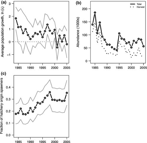
To evaluate impacts of changing flow regimes on the population growth of mid-latitude anadromous fish populations, we analyzed a dataset from the Puget Sound region (USA) of 21 populations of threate-ned Chinook salmon (Oncorhynchus tshawytscha) (Ford et al., 2010). In 1999, these populations were listed as threatened under the US Endangered Species Act, because natural origin fish were below 10% of historical levels (Myers et al., 1998; Gresh et al., 2000) (Fig. 1a). These Chinook populations occupy a diverse range of habitat areas (30 000 to 475 000 ha; Table 1), that vary in altitude, geologic characteristics, and human disturbances (Ruckelshaus et al., 2006). From the perspective of climate change, these habitats also range from rainfall-dominated (<790 m in elevation with peak discharge in December–February) to snowmelt-dominated (>1300 m elevation with peak discharge in May–June) systems (Beechie et al., 2006). Future climate projections in the region estimate warming trends to be 0.1–0.6 °C per decade, with expected increases in fall and winter rainfall (Mote & Salathe, 2010). Accordingly shifts in dominant discharge regimes are expected among the systems.
| River | Ln (growth) | 95% CIs | Area (km2) | USGS gauge | Δσ |
|---|---|---|---|---|---|
| Sammamish (R) | 0.82 | (0.38, 1.23) | 670 | 12125200 | 35%a |
| Cedar (R) | 0.96 | (0.54, 1.40) | 472 | 12119000 | −33%a |
| Dungeness (T) | 1.05 | (0.59, 1.49) | 521 | 12048000 | 30%a |
| Elwha (T) | 1.06 | (0.62, 1.49) | 839 | 12045500 | 24%a |
| Suiattle (S) | 1.07 | (0.64, 1.49) | 888 | NA | NA |
| Upper Sauk (T) | 1.12 | (0.7, 1.53) | 673.5 | 12186000 | 27%a |
| SF Stillaguamish (R) | 1.12 | (0.67, 1.53) | 665 | 12161000 | 22% |
| SF Nooksack (T) | 1.15 | (0.74, 1.57) | 479 | 12209000 | 20% |
| NF Stillaguamish (R) | 1.24 | (0.82, 1.66) | 752 | 12167000 | 4% |
| Skokomish (R) | 1.26 | (0.83, 1.69) | 643 | 12061500 | 27%a |
| Cascade (S) | 1.3 | (0.86, 1.72) | 490 | 12182500 | 32%a |
| NF Nooksack (S) | 1.34 | (0.91, 1.78) | 642 | 12205000 | 27%a |
| Lower Skagit (T) | 1.4 | (0.95, 1.84) | 2142 | 12200500 | 7% |
| Lower Sauk (T) | 1.41 | (0.96, 1.84) | 341 | 12189500 | 31%a |
| White (T) | 1.49 | (1.04, 1.91) | 1293 | 12098500 | 19% |
| Puyallup (R) | 1.49 | (1.06, 1.90) | 1409 | 12093500 | 16%a |
| Skykomish (T) | 1.53 | (1.08, 2.01) | 2179 | 12134500 | 24%a |
| Snoqualmie (R) | 1.65 | (1.23, 2.08) | 1802 | 12149000 | 15%a |
| Duwamish (R) | 1.73 | (1.18, 2.34) | 1296 | 12113000 | −20%a |
| Upper Skagit (S) | 1.9 | (1.26, 2.64) | 2717 | 12181000 | −24%a |
| Nisqually (R) | 1.95 | (1.46, 2.43) | 1974 | 12089500 | −49%a |
- a Δσ represents the percent change in the SD of differenced winter log(discharge), 1950–2012, with significant trends.
Materials and methods
Salmon data
We focused our analysis on data from 21 extant populations of Chinook in the Puget Sound region of Washington State, https://www.webapps.nwfsc.noaa.gov/. These populations are thought to be independent (Ruckelshaus et al., 2006), but small amounts of dispersal may cause their dynamics to operate as a meta-population. For each population, we used estimates of spawning adult numbers and age structure in each calendar year to reconstruct the population growth (adults produced per adult), 1984–2005. We focus exclusively on fish that spawn in the natural environment. There are extensive releases of artificially propagated (hatchery) juvenile Chinook salmon in these same rivers, however, and many of these released fish eventually return to the natural environment to spawn. Accounting for these external inputs to the natural spawning areas is therefore important for estimating the intrinsic growth rates of the natural populations. Numbers of natural spawning adults of hatchery and wild origin in each year were used to generate time series of the proportion of hatchery origin spawners, used as a covariate in our statistical model. The proportion of hatchery individuals in this ecosystem varies widely (0–97%) across populations and through time; because hatchery origin salmon have been shown to sometimes have lower reproductive success when spawning naturally than natural origin salmon (Araki et al., 2008), we allowed for differing productivity of hatchery and wild origin spawners (Buhle et al., 2009). Additional detail provided in the SI.
Environmental covariate data
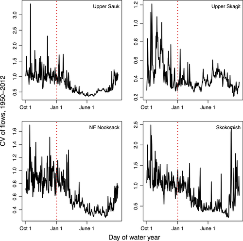
Raw river flow data were downloaded from the US Geological Survey stream gauges (http://www.usgs.gov/, Table 1). Mean and SD summary statistics were based on log-transformed daily winter flow data, Oct 1–Jan 31. Chinook salmon are generally classified as ‘ocean type’ (juveniles migrate to the ocean in their first year) and ‘stream type’ (juveniles spend a year rearing in freshwater), with the majority of Puget Sound Chinook being the former (Beechie et al., 2006). Ocean-type Chinook generally spawn in freshwater habitats in September, and juveniles surviving the winter migrate to the ocean 4–9 months later. Thus, October to February represents the earliest life stage of these salmon populations and the period of egg incubation during which the majority of lifetime mortality occurs (Quinn, 2005). Flow data in this period are also the most variable (Fig. 2) and potentially sensitive to impacts of climate change (Mote, 2003; Fig. 3). To calculate the SD of annual flows (our metric of variability), we first-differenced daily flow data after log-transforming, dt = log(yt+1) – log(yt). This transformation is widely used in time series analysis to stabilize the mean and variance (Shumway & Stoffer, 2006), but may be unfamiliar to many ecologists or hydrologists, but first-differenced logged values have a similar interpretation as rates of change. Mean flow was summarized as the average log-transformed flow over the winter period, and peak flow timing was calculated as the day of the largest winter peak flow event. For three rivers (Cedar, SF Stillaguamish, Suiattle), portions of the flow time series were missing – because we analyzed these data in a Bayesian framework, we treated these missing values as unknown parameters and integrated over the range of values. To ensure that these missing flow values did not affect our results or conclusions, we also reran our entire analysis with these three populations omitted. Additional details are provided in the SI.
To link ocean conditions to adult survival, we used the Pacific Decadal Oscillation (PDO) and North Pacific Upwelling (NPU) as covariates, because both have been previously linked to larger trends in salmon abundance or survival (Mantua et al., 1997; Scheuerell & Williams, 2005). PDO anomalies were downloaded as monthly summary statistics (http://jisao.washington.edu/pdo/), and we treated the May–September average as a predictor. Upwelling indices were downloaded as monthly data from the station closest to the Puget Sound region (http://www.pfeg.noaa.gov/products/pfel/modeled/indices/upwelling/upwelling.html) at 48N 125W. Unlike the metrics of river flows which were specific to each population, these metrics associated with the marine environment were included at a large scale, with all populations assumed to experience the same conditions.
Statistical model

 , flow variability, σt,j, and date of peak flow events, peakt,j) are linked to population growth via the coefficients fx, fσ, and fpeak. Finally, we included a trend parameter (u) to allow for changes not explained by our model.
The final terms in the model represent the variance, decomposed into spatial and non-spatial components. The term δt,j represents correlated error (environmental stochasticity). To account for the adjacent populations in our analysis potentially experiencing similar environmental conditions, we treated this stochasticity as being correlated between populations, δt,1:m ~ MVN(0,Σ). Elements of the covariance matrix Σ were modeled as an exponential function of pairwise hydrologic distances between populations, Σi,j = θ2exp(−ϕ|di,j|), where θ2 represents a variance parameter, ϕ represents a decay parameter, and di,j represents the pairwise distance between populations i and j (Cressie & Wikle, 2011). To account for non-spatial errors (e.g., residual error), we included an additional independent variance term. For Chinook salmon in Puget Sound, this additional estimated variance represents uncertainty in age structure, adult counts, and fishery harvest that are extrapolated to the population level. We assumed that this residual error was normal, so that Yt,j ˜ Normal(E[λt,j], σresid). All parameter estimation was conducted in a Bayesian framework (additional details about the salmon data and model provided in the SI).
Results
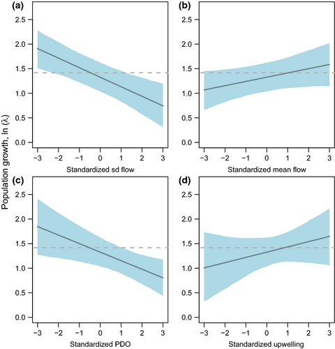
While the average growth rate across populations is greater than zero in most years, overall abundance of Puget Sound Chinook salmon has declined, even as harvest levels have decreased (Fig. 1a,b). The discrepancy between positive growth and declining abundance can be explained by average growth-weighting populations equally (instead of weighting populations in proportion to abundance). Of the freshwater and marine environmental variables considered as drivers of population growth, the strongest estimated effect on Chinook salmon was the negative relationship between Chinook population growth and variation in winter daily flows (Figs 2 and 3, Table 2). The effect of PDO was slightly more negative than flow variability; however, the 95% CIs of PDO are also overlapping 0 (thus would not be considered ‘significant’ in the classical interpretation). The remaining hydrologic variables (residualized mean flow, timing of peak flow) had 95% posterior credible intervals overlapping 0, indicating weak to negligible effects (Table 2). Variables related to ocean conditions were estimated to have contrasting effects on Chinook population growth that are largely consistent with previous work (Mantua et al., 1997; Greene et al., 2005; Scheuerell & Williams, 2005); PDO was estimated to have a weak negative effect, and Pacific upwelling was estimated to have a weak positive effect, but similar to mean flow and peak flow timing, the 95% intervals for both overlapped zero (Table 2, Fig. 4b–d). Estimates of population-specific growth rate parameters ranged from 0.81 to 1.89 and were highly correlated with basin areas (ρ = 0.74, P < 1e-5, Table 1). Hatchery-produced adult fish were estimated to have slightly depressed productivity (stronger effects of density dependence) relative to natural origin adults (Fig. S1). Because the 95% CIs of the difference overlapped zero (a result similar to Buhle et al., 2009), the effect would not be classically interpreted as significant. The final coefficient (u) representing temporal trends not explained by our model was estimated to be a negative decline of approximately 4% annually (Table 2).
| Coefficient | Estimate | 95% CIs |
|---|---|---|
| PDO (bPDO) | −0.219 | (−0.334, 0.051) |
| Upwelling (bNPU) | 0.129 | (−0.072, 0.274) |
| Mean annual flow (fx) | 0.092 | (−0.003, 0.179) |
| SD of annual flow (fσ) | −0.178 | (−0.286, −0.100) |
| Timing of peak flow (fpeak) | 0.044 | (−0.061, 0.119) |
| Time trend (u) | −0.043 | (−0.059, −0.025) |
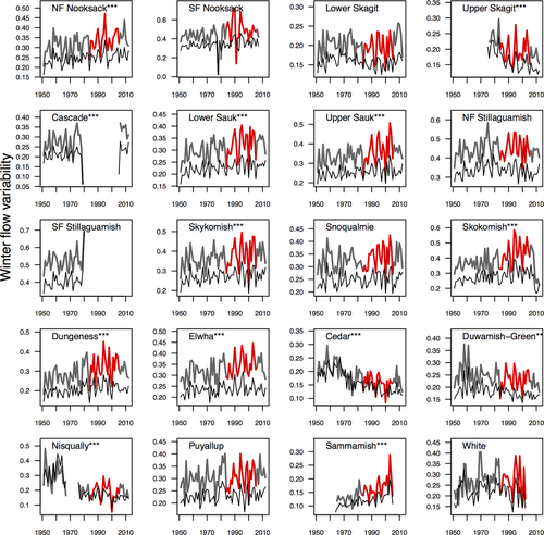
The negative correlation between productivity and variation in winter flows in the Puget Sound region is a cause for concern because since 1950, there have been increases in winter flow variation for 16 of 20 populations in our analysis (11 significantly so, P < 0.03; Fig. 3; Table 1). Populations with significant positive increases included two of three rivers previously identified as being snowmelt dominated (NF Nooksack, Cascade), five of nine rivers with transitional regimes (Lower and Upper Sauk, Skykomish, Dungeness, Elwha), and four of nine rivers with flows driven by rainfall (Snoqualmie, Skokomish, Puyallup, Sammamish; Beechie et al., 2006). To interpret trends in variance across rivers, we used variability in 1950 as a baseline; this indicated that for these 11 rivers, variation in flow has increased by 35% over 60 years (or 1.45 SDs, Table 1). In contrast to the trends in winter flow variation, no rivers have shown significant changes in mean winter flow, and only one has shown evidence of a change to earlier peak flow events (Snoqualmie). We also found four significant negative trends in flow variability (Table 1: Cedar, Duwamish, Upper Skagit, Nisqually).
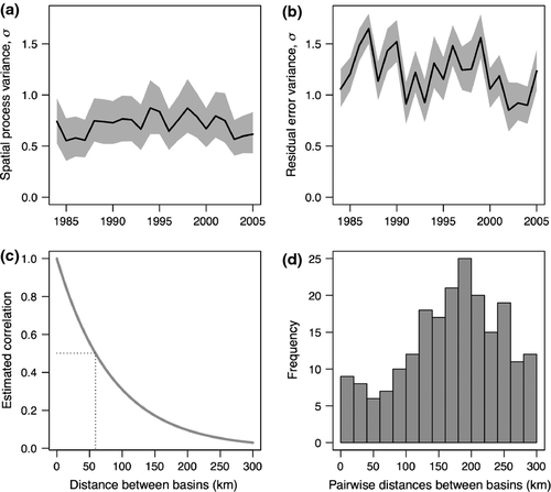
Populations separated in Puget Sound by <50 km are estimated to have correlated growth rates (ρ > 0.5; Fig. 5c,d), suggesting that any diversity in the response to the environmental variables in our model occurs between populations >50 km apart. After accounting for all of the environmental variables in our analysis, and changes in data quality over time related to residual error, there appears to be no trend in the variance of population growth over time for these populations, suggesting there has been no loss of portfolio buffering among populations from 1984 to 2005 (Fig. 5a). Instead, the residual variance appears to have decreased slightly over time (Fig. 5b), possibly related to either improvements in monitoring methods, or smaller populations that are easier to count.
Discussion
Globally, there is increased recognition of the importance of including effects of climate change in risk assessments and spatial planning in aquatic species (Mcclure et al., 2013). A challenge in conducting risk assessments for anadromous species, such as Chinook salmon, is that climate change may act directly or indirectly on the species in more than one ecosystem (e.g., marine, freshwater, or terrestrial environments). Moreover, species with strong aquatic-terrestrial linkages, like Chinook salmon (Helfield & Naiman, 2001), highlight the need for management and conservation actions that consider cost-benefit tradeoffs across coupled ecosystems.
While understanding species response to directional changes induced by climate change is important, our study highlights the importance of also considering impacts of ecosystem variability. Over the last half century, river flows included in our analysis have become more variable – particularly in winter (Figs 2 and 3) – and these changes are a stronger predictor of Chinook population growth than changes in average winter flows (Fig. 4b), or climate signals in the marine environment (Fig. 4c,d). While other impacts to this ecosystem, such as habitat degradation, may be hypothesized as responsible for these trends in flow variation, we found support for increasing flow variation in high-altitude rivers with relatively low human impacts (Fig. 3: Cascade, Upper Sauk, NF Nooksack). One potential mechanism for the relationship between flow variability and population growth rate is that Chinook salmon spawn at relatively low flows during the late summer or early fall, and later peak flows during winter can scour eggs from the gravel (DeVries, 1997). As flow variation increases, the likelihood of egg loss increases because lower spawning flows encourage egg deposition nearer the center of the channel as fish seek water of sufficient depth for nest construction, and the highest probability of scouring during peak flows is in mid-channel (Haschenburger, 1999). As the frequency of fall and winter storms in the Pacific Northwest is expected to increase, the trend in increased variation in winter flows is projected to continue (Mote & Salathe, 2010), potentially decreasing productivity through increased mortality during the egg incubation stage.
The effect of increased flows may not be entirely negative, however. Although the 95% credible intervals overlap 0 (and thus the effect would not classically be interpreted as ‘significant’), we estimated a slight positive relationship between mean winter flow and Chinook salmon productivity. Mechanisms that may lead to a positive effect include reduced predation on juveniles in more turbid environments (Gregory & Levings, 1998) or benefits to juveniles that overwinter (Sommer et al., 2005). Another possibility is that wet summers followed wet winters, which may have benefited stream-type Chinook salmon that rear in streams for more than a year. Our selection of flow predictors only focused on the dominant ocean-type life history type in the region, but survival of the less common stream-type Chinook may suffer during years of extreme low summer flows.
The marine indicators were weaker predictors of Puget Sound Chinook salmon productivity than stream flow variability, a result in agreement with other recent studies. In an analysis of 24 stocks of Chinook salmon ranging from central California to southern Alaska, Sharma & Liermann (2010) also found a weak negative effect of PDO on recruitment with posteriors that overlapped zero, similar to the results of our study. Covariation of marine survival patterns across North America suggests Chinook salmon may respond to marine conditions at multiple spatial scales, including variation in the local marine environment (Sharma et al., 2013). Like the effect of PDO, our analysis found a weak association between salmon productivity and coastal upwelling estimated in the California Current off the Washington Coast. In contrast to these broader marine signals representing the conditions of the entire NE Pacific, Greene et al. (2005) found that a large proportion of Skagit River Chinook salmon adult recruitment was explained by fine scale variation in the estuary and nearshore marine waters. After accounting for all of the environmental variables in our analysis, our results indicated that growth of these populations continues to have a declining trend, not attributable to factors in our model. These other potential factors may include the effect of contaminants, competition with other fish species, and increased predation by marine mammals.
Although our analysis is concentrated on how changes in climate variability affect mean population growth rates, our model also allows us to examine effects of climate variables on changes in the variation of population growth rates. Asynchrony of salmon populations has been recognized as a ‘portfolio effect’ whereby populations responding differently to dynamic environmental conditions increase resilience, persistence, and economic value of the aggregate (Moore et al., 2010; Schindler et al., 2010). Our statistical approach advances this line of research by explicitly accounting for changes in residual error, permitting a more direct assessment of the variance in ecological processes governing salmon population dynamics. Because we also consider the variability among populations through time, we can address temporal changes in variance over short time periods. In this case, Chinook salmon in Puget Sound show little change in portfolio variance over our 30 year time series (Fig. 5a), but greater variation (and slight trend) in the residual variation. This result highlights the need for incorporating changes in data quality in long-term ecological analyses, particularly as new methods and technology are used in data collection.
Focusing on the winter period, October–January, it is unlikely that management actions can reverse trends of basins transitioning from snowmelt-dominated to rainfall-dominated hydrographs (Beechie et al., 2006) or the frequency of rain on snow events. Management actions that focus on restoration of Chinook salmon spawning, and juvenile rearing habitat in winter may be most successful. Actions that may buffer increasing flow variability in the Pacific Northwest include reconnection of floodplains that can enhance flood storage capacity and provide refugia habitat for juvenile fish, increasing lateral connectivity to floodplain aquifers, and reducing delivery of runoff from impervious surfaces into streams (Battin et al., 2007; Beechie et al., 2013). Restoration activities may increase Chinook salmon survival and productivity in local watersheds, but also have rippling effects through marine systems, creating future economic value through their role in the food web (for example, serving as prey to marine mammals) and via commercial and recreational fishing opportunities.
Acknowledgment
The authors thank K.N. Marshall, C.E. Jordan, M. Rowse, and 2 anonymous reviewers for providing helpful comments for earlier versions of this work.


