Fatigue failures from defects in additive manufactured components: A statistical methodology for the analysis of the experimental results
Funding information: CAS Pioneer Hundred Talents Program; National Natural Science Foundation of China, Grant/Award Numbers: 11872364, 12072345, 11932020
Abstract
The fatigue response of additive manufactured (AMed) components is generally controlled by the defect population, and the models for assessing the fatigue response of AMed parts have to take into account the distribution of defect size and the intrinsic scatter associated to the fatigue response. In the present paper, a statistical methodology for analyzing the results of tests on AMed specimens failed due to cracks originating from defects is proposed. The procedure involves the estimation of the distribution of the fatigue life, which is considered dependent on the applied stress amplitude and on the defect size. Thereafter, all the experimental failures are shifted at a reference number of cycles to failure or stress amplitude, making it possible to compare data obtained at different stress levels or number of cycles to failure. The proposed method has been successfully validated on literature dataset, proving its effectiveness and general validity.
1 INTRODUCTION
The diffusion of components produced through additive manufacturing (AM) processes has significantly increased in the last few years. Several AM components, like brackets,1-4 heat exchangers,5 and biomedical implants,6 can be employed in industrial applications to replace components produced through traditional processes. In particular, if only quasi-static loads are applied, they can be safely employed and designed by considering the results of tensile tests, as for traditionally built parts. Indeed, the tensile strength of AM parts is generally close to that of parts produced through traditional processes, despite the different manufacturing processes and the different microstructures. Moreover, the scatter associated with the quasi-static tensile properties is generally limited,7-9 thus ensuring a safe use of AM components when subjected to static stress.
On the other hand, for applications in which fatigue loads are present, components produced through traditional manufacturing processes are still preferred. The main reason for the limited diffusion of AM parts in these applications is the worse fatigue behavior of AM parts, if compared to that of traditionally built components. Indeed, during the layer-by-layer process in AM, characterized by local fusions of the unmelted powder with different heating sources (laser for the laser powder bed fusion, L-PBF, process and electron beam for the electron beam powder bed fusion, EB-PBF), many defects originate within the material volume. Porosities, lack of fusion defects, and defects due to incomplete bonding10 can form within the component material and represent an ideal site for the crack formation, inducing a consequent premature failure. For these reasons, the fatigue response of AM parts is typically worse than that of traditionally built parts, which are generally free of large defects with sizes comparable to those of AM parts.9-14 The aim of the research is therefore to optimize the process parameters or the post-treatments in order to limit the formation of defects15, 16 or to define damage tolerance design approaches capable to ensure the structural integrity of AM parts, since the design procedure commonly adopted cannot be conservative and effective.13
In order to properly compare the results of tests on AM parts and assess the influence of process parameters and post-treatments, the experimental data should be properly analyzed. According to the literature, the fatigue crack originates from the most critical defect within the material volume, which generally corresponds to the largest defect.17, 18 Defects are randomly distributed within the material volume, and the scatter associated with their size is very large. Consequently, the scatter of the fatigue response for AM parts is large,9, 15, 19 making it difficult to analyze the experimental data and to assess the influence of the investigated factors, as they can be “hidden” by the experimental scatter. Therefore, the experimental data should be analyzed with appropriate statistical methodologies capable of taking into account, together with the defect size, also the experimental scatter. It is clear that a proper analysis would require a large experimental dataset: however, the number of available AM specimens is generally smaller than that for traditionally built specimens, due to their high production cost. Therefore, especially if the effect of a specific factor is investigated and a small number of failures at different stress amplitude is available, the analysis can be difficult and the results of difficult interpretation. The development of statistical methodologies capable of maximizing the information contained in the experimental data is therefore crucial for a proper analysis of the results of tests on AM parts.
In the present paper, a statistical methodology for analyzing the experimental results of tests on AM specimens is proposed. The procedure involves the estimation of the distribution of the fatigue life and, thereafter, to shift all the experimental failures at a reference number of cycles to failure or reference stress amplitude. With all the data at the same number of cycles to failure (or stress amplitude), different statistical methods can be applied to analyze the data and assess the factors that are significant for the fatigue response. In the first part of the paper, a general model for the fatigue life in presence of defects is presented, and the procedure for shifting all the data at the reference number of cycles to failure or stress amplitude is described. In the second part of the paper, the proposed statistical method is validated on experimental datasets available in the literature, proving its validity and effectiveness.
2 MATERIALS AND METHODS
The present section describes the statistical methodology employed for the analysis of AM fatigue data. In Section 2.1, the general statistical model for the fatigue life is introduced. In Section 2.2, the proposed statistical methodology for the analysis of the experimental data is presented and described, as well.
In the following, the subscripts H and V refer to the HCF and the VHCF region, respectively. Therefore, the coefficients with subscript H and V refer to the models for the fatigue life in the HCF region and in the VHCF regime, respectively.
2.1 Fatigue failures in presence of defects: General model for the PSN curve
For a safe design of components subjected to fatigue loads, an appropriate experimental assessment of the material response with respect to the number of cycles is fundamental. For this reason, the S–N curves, that model the variation of the fatigue life, or the number of cycles to failure, with respect to the applied stress amplitude, are widely adopted. In a probabilistic framework, the statistical distribution of the fatigue life can be also attained, since the fatigue phenomenon is intrinsically characterized by a large scatter that must be carefully taken into account when components are to be designed. International standards prescribe how to analyze the fatigue test results and to assess the distribution of the fatigue life up to the High Cycle Fatigue (HCF) regime.20 Moreover, in order to model the fatigue response of parts also in the Very High Cycle Fatigue (VHCF) regime, different models have been proposed in the literature.21-25 If the fatigue failure originates from manufacturing defects, the influence of the defect size on the fatigue life distribution should be also considered.17, 26
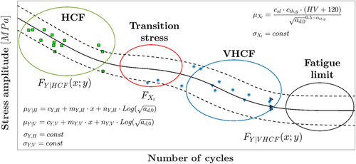
Starting from the models proposed by Paolino et al,22, 26 a general model for the fatigue life in the HCF region and in the VHCF region can be defined, permitting the estimation of the so called “duplex PSN curves.”23, 24 It involves a first linear decreasing trend in the HCF region, a transition stress, and a second linear decreasing trend in the VHCF regime ending with a horizontal asymptote (i.e., the fatigue limit). Moreover, the dependency between the fatigue life and the defect size distribution is also included in the model.
 (1)
(1) is the cdf of the transition stress between HCF and VHCF region, and FY|HCF(y; x) and FY|VHCF(y; x) are the marginal cdf of the fatigue life in the HCF region and in the VHCF region, according to Paolino et al.26 The transition stress is assumed to follow a normal distribution, that is,
 , with constant mean
 and standard deviation
 (Φ(·) is the cdf of a standardized Normal distribution).
 (2)
(2) the cdf of the conditional fatigue life (i.e., the fatigue life conditioned to the defect size),
 the cdf of the fatigue limit, and
 the truncated probability density function (pdf) of the defect size
 (assumed as the projected area of the defect in a direction perpendicular to the load direction, according to Murakami17).
 is assumed to be normally distributed, with mean
 depending on x and
 and constant standard deviation σY,V.
 is also assumed to be normally distributed, with mean
 dependent on the material Vickers hardness and on
 and constant standard deviation
 For more details on the model, the reader is referred to Paolino et al.26 According to Murakami,17 the defect size
 is assumed to follow a Largest Extreme Value Distribution (LEVD). In particular, a truncated (to 0) distribution of the LEVD is assumed, since the defect size
 cannot be negative.27 According to Equation 2, the marginal distribution of the fatigue life does not depend on the defect size.
The expression for the marginal cdf of the fatigue life in the HCF region (or due to a first failure mode) is the same of Equation 2, but in this case, the distribution of the fatigue limit is obviously not considered (i.e.,

 )). It is worth to note that the distribution of the fatigue life and of the defect size is different for the HCF region and for the VHCF region (i.e., the constant parameters of the distribution are different for the HCF region and the VHCF region).
Equations 1 and 2 permit to model the so-called “duplex S-N curve,” according to Wei et al. and Kikuchi et al.23, 24 The general model can be also modified to consider simpler cases. For example, if the fatigue limit is not present, the model in Equation 1 is modified by considering
 . On the other hand, if the experimental data follow one linear trend ending with fatigue limit,
 in Equation 1 is equal to 0.
Figure 1 shows a typical example of a duplex probabilistic S–N (PSN) curve with the statistical models considered for modeling the fatigue life. The expressions for the mean of the finite fatigue life distribution in the HCF and in VHCF region and of the fatigue limit, introduced in Equations 1 and 2, are also reported. The constant parameters involved in the models for the finite fatigue life in the HCF region and for the finite and infinite (i.e., the fatigue limit) life in the VHCF region are estimated separately, according to the procedure described in Paolino et al.26 Given these coefficients, the mean and the standard deviation of the transition stress distribution are estimated by maximizing the likelihood function of the model in Equation 1, so that both failures and run-out specimens can be considered. Alternatively, all the unknown parameters can be estimated by maximizing the likelihood function of the complete model. In this case, however, the number of parameters to be estimated is large, and the choice of the initial values for the parameters to be estimated can be difficult (e.g., by using the function fminsearch of MATLAB® that adopts the Nelder–Mead simplex algorithm). From Equation 1, the α quantile of the PSN curve can be estimated by substituting FY(y; x) with α and numerically solving Equation 1 with respect to x for different values of y. Therefore, for each value of y in the selected range of number of cycles to failure, the x value of the αth quantile curves is obtained by numerically solving Equation 1, since a closed-form solution does not exist. From a practical point of view, y can be iteratively varied in the range of interest to obtain the corresponding xα for the the αth quantile curves. Given y and xα, the α quantile of the PSN curve can be built on an S–N plot. Generally, the authors use the fzero function in a MATLAB® code to define the PSN curves.
2.2 Fatigue failures in presence of defects: Statistical methodology
The number of AM specimens for fatigue tests is generally smaller than that available for traditionally built specimens, due to the high cost of the AM processes and powders. Therefore, the information contained in the experimental dataset should be “maximized,” by properly accounting also for the large scatter of fatigue data, mainly associated with the random distribution of the defect size. In this respect, if the fatigue tests are carried out at different stress levels and, for each level, the number of results is limited, it might be difficult to analyze the fatigue data (or to assess the influence of a specific factor). The analyses, on the contrary, could be more effective if all the data are gathered together at a defined number of cycles to failure (or stress amplitude) which is considered as representative of the fatigue life: In this way, also the scatter associated with the experimental data can be properly taken into account.
In order to “shift” all the experimental failures to a defined number of cycles to failures (in the following, denoted as reference number of cycles, Nref) or to a defined stress amplitude (in the following, denoted as reference stress amplitude, sref), Equation 1 can be exploited. Figure 2 shows graphically the procedure for assessing, for each experimental failure, the corresponding failure at Nref or sref. As a representative example, the case of a PSN curve with a decreasing trend and a fatigue limit is shown.
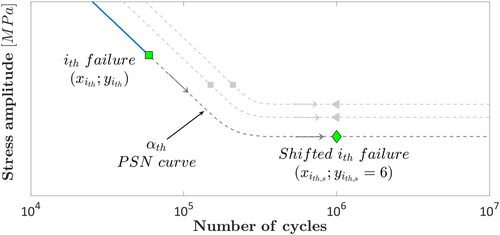
According to Figure 2, a specific PSN curve passes through each experimental datapoint: It is worth to note that this is true only if the parameters of the distribution of the fatigue life are properly estimated and are close to the actual values. For example, the ith failure (square gray marker in Figure 2, with coordinates (yith; xith)) is crossed by the PSN curve characterized by the failure probability αth (i.e., FY(y; x) = αth). By following the PSN curve with αth failure probability, it is therefore possible to assess for the ith failure the corresponding failure at Nref or sref (the gray diamond marker in Figure 2 is the ith failure at Nref = 106 cycles). By repeating this procedure for all the experimental failures, it is possible to gather all the data and to properly compare them with statistical methodologies, like the analysis of variance (ANOVA) or the hypothesis test. In this way, the scatter associated with the experimental data can be properly taken into account, since the influence of a factor can be “hidden” or overestimated due to the experimental large scatter.
For the sake of clarity, in order to shift all the experimental data, the unknown parameters of the model in Equation 1 (or of a simplified model, depending on the experimental dataset) are to be estimated according to the procedure described in Section 2.1. Given the unknown parameters, the model for the fatigue life is completely defined. For the ith failure (gray square marker in Figure 2), the logarithm of the number of cycles to failure and of the applied stress amplitude (yith and xith, respectively) is known and can be inserted in Equation 1, which can be solved to find the αth PSN curve (blue curve in Figure 2) that crosses the ith failure. In other words, each point on the αth curve permits to assess the stress amplitude characterized by a probability of failure equal to αth. Therefore, given αth, the stress amplitude
 for the ith failure shifted at a larger number of cycles to failure (e.g.,
 in Figure 2, green diamond marker) can be easily obtained by numerically solving Equation 1.
From a practical point of view, the proposed methodology can be applied only if the constant coefficients involved in Equation 1 are properly estimated. Therefore, for each experimental failure, the stress amplitude, the number of cycles to failure, and the defect originating failure should be known. By properly modifying Equation 1, the proposed procedure can be also applied without knowing the defect sizes. However, in this case, the information concerning to the influence of defects is missed.
3 VALIDATION ON LITERATURE DATASET
In this section, the proposed procedure has been applied to experimental datasets taken from the literature for which it was possible to extrapolate, for each failure, the number of cycles to failure, the stress amplitude, and the defect originating the fatigue failure (critical defect in the following). Run-out specimens, for which the largest defect was reported (e.g., by testing them at higher stress amplitude), have been also taken into account in the analyses. The software Engauge Digitizer was used to digitalize the data points reported in the figures of the analyzed papers, if not available in any specific table. It is worth to note that the digitization of the experimental dataset from the figures reported in the analyzed paper can be affected by possible errors. However, the main objective of the paper is to validate the proposed statistical methodology, and small errors in the digitization can be accepted. The influence of the digitalization error is larger for small datasets: However, in all the analyzed cases, the number of data is enough to obtain reliable results. Moreover, the possible influence of digitization errors has been verified, by algebraically adding a random uncertainty to the retrieved experimental data. The digitization uncertainty has been estimated by considering the range of possible values when extracting the values in the picking phase (e.g., by picking the points just outside the symbols). Even by considering a large uncertainty, the results obtained and reported in the following section are confirmed, with the digitization uncertainty having a limited influence.
Depending on the experimental data, different models have been considered (e.g., monotonic decreasing trend or decreasing trend ending with a fatigue limit), finally choosing the one providing the best fit. For the parameter estimation, the strategy providing the best fit was considered. The analyses have been carried out by shifting the experimental failures at a reference number of cycles to failure. The reference number of cycles to failure has been chosen as:
- the number of cycles for which the fatigue life is infinite (i.e., an Nf on the part of the curve showing an asymptotic trend, for the experimental dataset showing a fatigue limit),
- the run-out number of cycles to failure, if available, or 2 · 106 (i.e., a typical number of cycles to failure in the HCF region)
- the Nf considered by the authors of the original papers.
For duplex PSN curves, on the other hand, the transition stress distribution has been analyzed.
For the sake of clarity, the analyzed experimental dataset are subdivided by the material type. In the following, “X-Y building direction” refers to specimens built with their axis parallel to the building platform, whereas “Z building direction” refers to specimens built with their axis perpendicular to the building platform.
3.1 Titanium alloys
The influence of defects on the fatigue response up to Nf = 2 · 106 cycles of a grade 23 ELI TA6V alloy used in medical and aeronautical applications was investigated in Le et al.28 Standard dog bone specimens for the fatigue tests were obtained after a machining process of samples (200 μm removed) produced with an SLM280 HL machine. Before the machining process, the specimens were heat-treated (annealing at 850 ° C for 2 h and furnace cooling) to remove residual stresses. The fatigue tests were carried out with R equal to 0.1, and the effect of the building orientation was investigated by producing specimens in the XY direction, at 45° with respect to the building platform and in the Z direction. The S–N plot reported in Le et al.28 depicts the maximum stress, normalized with respect to the average value of the ultimate stress in the three building directions, with respect to the number of cycles to failure: In the following analysis, the normalized data are considered. Moreover, two batches for the XY building orientation, three batches for the 45° building orientation and two batches for the Z building orientation were considered (i.e., all batches were obtained with the same process parameters) to investigate the fatigue response scatter. For each building orientation, Bx refers to the x batch (e.g., B1 refers to the first batch).
For the analysis of the experimental data, the model involving the presence of the fatigue limit at the end of the curve was considered for all the dataset, according to Le et al,28 apart from the batch B3 (45° building orientation) for which a clear fatigue limit cannot be estimated from the experimental data. Figure 3A plots, for each building orientation and batch, the fatigue strength at the reference Nref = 107 cycles (i.e., all the experimental failures have been shifted to Nref = 107 cycles). For each batch, the estimated fatigue strengths at 107 cycles are reported within the round brackets; whereas, the σmax0,n in Le et al.28 (i.e., the horizontal asymptote of the curve) is reported within the square brackets. In Figure 3B, the data points at Nref = 107 cycles have been grouped to assess the influence of the building orientation on the fatigue response.
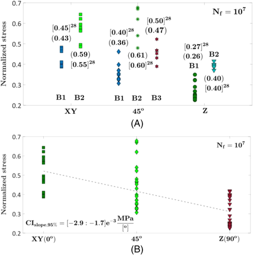
According to Figure 3A and in agreement with the analysis in Le et al,28 the scatter associated with the batches is large, even if the same process parameters were considered. Indeed the defect sizes vary among the batches, thus inducing significantly different fatigue responses. The normalized fatigue strength at 107 cycles estimated with the model reported in Equation 1 (median value reported in round brackets) is close to the fatigue strength reported in Tab. 3 in Le et al.28 (square brackets in the Figure), thus confirming that the proposed model is appropriate in assessing the influence of defects on the fatigue life. In addition, by shifting all the experimental failures at 107 cycles, it is possible to statistically compare failures occurred at different number of cycles, adding more strength to the analysis. For example, for each building orientation, an ANOVA analysis has been carried out to assess the influence of the batch variability on the fatigue response. The fatigue strength of the batches varies significantly for each building orientation, as the p value for each ANOVA is equal to 0. By shifting and grouping all the data together, it has been possible to assess the batch variability given the large scatter associated with the experimental failures. Therefore, in agreement with the conclusions of Le et al,28 this analysis confirms that the variability between different batches can be large, even if the specimens are produced with the same process parameters.
In Figure 3B, the effect of the building direction is investigated by grouping all the data for each building orientation. It is worth to note that the large scatter could hide the effect of this factor: However, since the same process parameters were used for manufacturing all the specimens, all the data coming from different batches must be considered together. Otherwise, the scatter associated with the AM process is neglected, obtaining less reliable results and missing important available information. As highlighted by the authors, a clear tendency between the specimens built in the XY directions and at 45° is not observed: Indeed, by carrying out an ANOVA between these two building orientations, the p value is 6.2%, larger than a typical 5% significance level, confirming the obtained results. Moreover, the specimens built in the Z directions are characterized by the smallest fatigue strength. However, if all the experimental data are considered together and an ANOVA is carried out, the building orientation is confirmed to be a statistically significant factor, with p value equal to 0. A linear interpolation between the fatigue strength and the building angle (0°corresponds to the XY building direction and 90° corresponds to the Z building direction) has been also carried out in Figure 3B: The slope of the curve is negative, and the 95% confidence interval for the slope does not contain the zero value, proving that the fatigue strength significantly decreases with the building angle. It can be concluded that, according to Le et al,28 the building orientation strongly affects the fatigue response, with the fatigue strength being larger for XY and the 45° and decreasing significantly for the Z building direction.
The influence of defects and manufacturing processes on the fatigue response of Ti6Al4V specimens has been also investigated in Masuo et al.29 Dog bone specimens were produced through a Direct Metal Laser Sintering (DMLS) and an Electron Beam Melting (EBM) process and subjected to different types of post-treatments. Rotating bending fatigue tests were carried out up to 107 cycles (runout number of cycles).
The experimental data obtained on specimens subjected to a surface polishing process (with #600 emery paper) and not subjected to the hot isostatic process (HIP) process are considered in the following analysis. The influence of the manufacturing process, DMLS and EBM, on the fatigue response is investigated. A model involving a decreasing linear trend and a fatigue limit was considered for the fatigue life. Figure 4A compares the cdfs of the fatigue strength at 107 cycles; in Figure 4B, the empirical cumulative distribution function (ecdf) of the difference between the fatigue strengths at 107 cycles obtained by testing the specimens produced through the DMLS and the EBM processes is plotted. In order to compute the ecdf for each manufacturing process, 1000 random values of the fatigue strength at 107 cycles have been simulated according to Equation 1 and by considering the parameters estimated according to the procedure reported in Section 2.2.
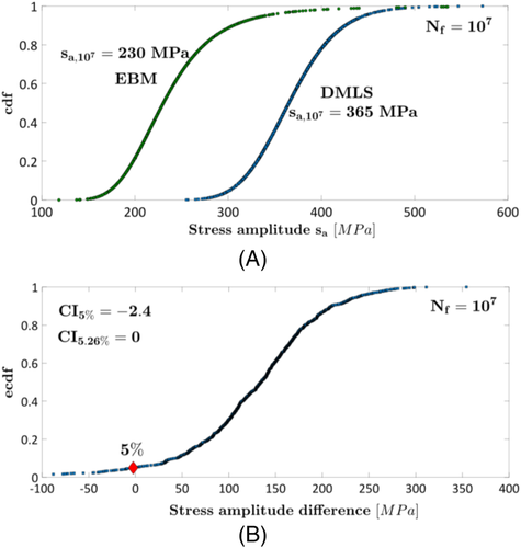
According to Figure 4A, the median fatigue strength at 107 cycles for the DMLS is larger (365 MPa for the DMLS specimens and 230 MPa for the EBM specimens) and close to the value obtained in Masuo et al.29 (fatigue limit equal to 370 MPa for the DMLS specimens and in the range [240 − 260] MPa for the EBM specimens). In order to assess if the fatigue strength of the DMLS specimens is larger, the ecdf of the difference between the fatigue strength has been computed and plotted in Figure 4B. According to Figure 4B, the difference is not statistically significant for a 5% significance level (ecdf equal to −2.4). However, a zero difference corresponds to an ecdf value equal to 5.26%, slightly larger than 5%. Therefore, due to this limited difference, it can be concluded that the fatigue response of specimens produced through the DMLS process is better than that of the specimens produced through EBM, in agreement with the results in Masuo et al.29
In Günther et al,30 the VHCF response of a Ti6Al4V alloy produced through different AM processes and the effect of post-treatments have been experimentally assessed. In particular, raw cylinders were produced through an SLM and an EBM processes and then machined to obtain the specimens for the ultrasonic (loading frequency of 19 kHz) fully reversed tension–compression fatigue tests. The specimens produced with the SLM process were subjected to different treatments: The specimens within the batch SLM-1b were subjected to a heat treatment involving a heating temperature of 800 ° C, whereas the specimens in the batch SLM-2 were subjected to hot isostatic pressing (HIP) at 920 ° C for 2 h at 1000 bar in an argon atmosphere. The EBM specimens were not subjected to posttreatments.
Figure 5 compares the pdf of the VHCF strength at Nref = 3 · 109 cycles for the three tested batches in Günther et al.30 A monotonic decreasing trend without fatigue limit was considered to model the fatigue life.
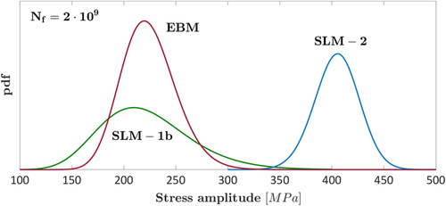
According to Figure 5, the production process and the subsequent post-treatments significantly affect the VHCF response of the investigated Ti6Al4V specimens, in agreement with the analyses in Günther et al.30 In particular, the VHCF response at Nref = 3 · 109 is about the same for the SLM-1b specimens (produced through SLM and heat-treated at 800 ° C) and the specimens produced through EBM. On the other hand, an HIP process permits to enhance the VHCF response. The trend is clear in Figure 5 and is further confirmed through an ANOVA of the experimental failures shifted at Nref = 3 · 109 cycles. The difference in fatigue strength is statistically significant by comparing the batches SLM-2 and the batches SLM-1b and EBM (p value close to 0), whereas it is not significant by comparing the VHCF strengths for the EBM and the SLM-1b batches (p value of 47.4%).
3.2 Aluminum alloys
In this section, the experimental results on aluminum alloys available in the literature are analyzed. In Qian et al,31 ultrasonic fatigue tests were carried out on AlSi10Mg specimens produced through an SLM process to investigate the effect of the stress ratio and of the building direction up to 109 cycles. Fatigue tests were carried out at a load frequency of 20 kHz on specimens produced in the XY and in Z direction and at stress ratio R equal to −1, 0 and 0.5.
For each experimental failure, the fatigue strengths at Nref = 109 cycles were estimated by considering a monotonic decreasing trend for the fatigue life. Figure 6A compares the VHCF strength at Nref = 109 cycles for the investigated building orientation and stress ratio. In Figure 6B,C the Haigh diagrams were estimated by considering a Goodman model passing through the 0.1% fatigue strength for a stress ratio equal to −1 and the tensile properties reported in the paper.31 In Figure 6D, the effect of the building orientation on the VHCF strength for different stress ratios is shown: For each stress ratio, the p value associated to the ANOVA, carried out to assess the influence of the building orientation, is reported.
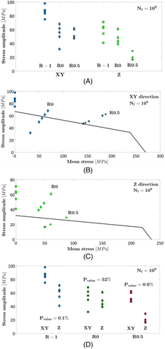
According to Figure 6A and as for the specimens produced with traditional manufacturing processes, the stress ratio has a significant influence on the VHCF strength for both the building orientation, with the fatigue strength decreasing as the stress ratio increases. This is confirmed by analyzing the Haigh diagram estimated in Figure 6B,C for the XY and the Z building orientation, respectively. Indeed, the Haigh diagram estimated by considering the 0.1% fatigue strength for R = −1 is in agreement with the experimental results, even if some failures occurred within the “safe region.” This could be due to the large scatter of the experimental data, associated with the random distribution of the defect size and to the limited number of experimental failures. However, this analysis provides a qualitative indication on the effect of the stress ratio, and this was possible thanks to the possibility of gathering all the experimental failures with the proposed methodology. A detailed analysis on the effect of the building orientation and on possible interactions between the stress ratio and the building orientation has been also carried out, according to Figure 6D. For each stress ratio, the experimental failures for the different building directions have been compared. It is found that the building orientation significantly affects the VHCF response for a stress ratio equal to −1 and 0.5 (p value close to 0), whereas it has no significant effects for a stress ratio of 0. An ANOVA considering all the experimental data at 109 cycles has been also carried out. As expected, the building orientation and the stress ratio significantly influence the VHCF response, as the p value is equal to 0. The interaction between the building orientation and the stress ratio has also been found to be significant (p value of about 0.8%). Indeed, depending on the stress ratio, the building orientation has a different effect on the VHCF response. This result can be due to the small number of available experimental results, and further analysis with a larger dataset should be carried out. For example, if the same ANOVA is carried out without considering the experimental results obtained with tests at a stress ratio of 0.5, the p value for the interactions increases to 5.1%.
In Tang and Pistorius,32 the effect of the building direction and of the hatch spacing on the fatigue response in the HCF region of an AlSi10Mg alloy was investigated. Standard dog bone specimens were produced through an SLM process and tested at a stress amplitude of 80 and of 100 MPa (stress ratio of 0.1). The specimens were built in the XY and in the Z direction: For each building orientation, three batches of specimens were produced with three hatch spacing (0.16, 0.19, and 0.22 mm). After the AM process, the specimens were heat-treated at 300 ° C for 2 h, to minimize the residual stresses, and thereafter machined to the final geometry.
A linear decreasing trend (without fatigue limit) was considered for modeling the fatigue life: Thereafter, all the experimental failures have been shifted to 2 · 106 cycles. Figure 7A,B shows the fatigue strengths at 2 · 106 cycles for the investigated building direction and hatch spacing, with the former focusing on the effect of the hatch spacing and the latter on the effect of the building orientation. Figure 7C,D compares the pdf of the fatigue strength for the XY and Z building orientation, respectively.
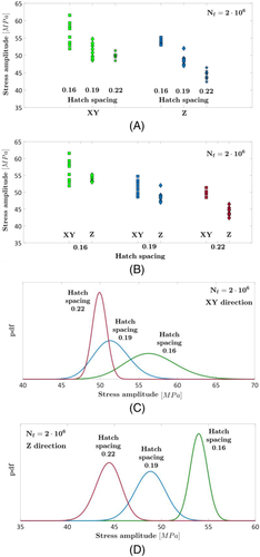
According to Figure 7A,C,D, the hatch spacing has a significant influence on the fatigue response, with the fatigue strength decreasing with the hatch spacing for both the building orientation, in agreement with the analyses carried out by Tang and Pistorius.32 However, differently from Tang and Pistorius,32 the proposed method permits to gather failures that occurred at different stress amplitudes, thus increasing the statistical significance of the analysis.
The building orientation also influences the fatigue response, especially for a hatch spacing of 0.19 and 0.22 mm. In order to investigate if the interaction between the building direction and the hatch spacing is significant, an ANOVA considering all the experimental data and the factors “hatch distance” and “building orientation” has been carried out. The results of the ANOVA are reported in Table 1: the sum of squares (SS), the degrees of freedom (DOF), the mean squares (MS), and the estimated p values are reported.
| SS | DOF | MS | p value | |
|---|---|---|---|---|
| Hatch distance | 546 | 2 | 273 | 0.000 |
| Building orientation | 152 | 1 | 152 | 0.000 |
| Interactions | 26 | 2 | 13 | 0.035 |
| Error | 152 | 43 | 3.54 | |
| Total | 865 | 48 |
According to Table 1, the hatch distance and the building orientation significantly affect the fatigue response of the investigated AlSi10Mg alloy, as the p value is close to 0. Furthermore, the interaction is statistically significant with p value equal to 3.5%. In general, for larger hatch distances, the effect of the building orientation seems to be larger, as shown in Figure 7A,B.
3.3 Maraging steel
In Meneghetti et al,33 the influence of defects on the fatigue response of a maraging steel was experimentally assessed. In particular, the specimens were produced in the XY and in the Z directions and tested without performing heat treatments, after a polishing process with progressively finer emery paper from grade 80 up to grade 800. The specimens were subjected to fully reversed (R = − 1) axial fatigue tests with a servo-hydraulic testing machine.
According to Meneghetti et al,33 a linear decreasing trend was considered for modeling the fatigue life. Figure 8A reports the experimental dataset in an SN plot, together with the estimated median and 1% PSN curves for the two investigated building orientation. Figure 8B,C compares the estimated fatigue strengths at Nref = 30,000 and Nref = 2 · 106 cycles, respectively.
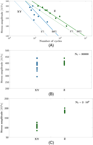
According to Figure 8A, the slope of the PSN curves is significantly different, being larger for the PSN curves estimated for the specimens produced in the XY direction, in agreement with the analyses carried out in Meneghetti et al.33 Accordingly, the effect of the building orientation depends on the number of cycles to failures, as proved Figure 8B,C. The fatigue response at 30,000 cycles (Figure 8B) for the two building orientations is similar (p value of 11% through an ANOVA); whereas, it is significantly different for a number of cycles to failure Nref = 2 · 106 (p value of 0). The dependency between the fatigue response and the building orientation can be also demonstrated with an ANOVA by considering all the experimental failures at 30,000 cycles and at 2 · 106 cycles (factors “building orientation” and “number of cycles to failure”). The building orientation and the number of cycles to failure have been found to significantly affect the fatigue response, as expected (p value equal to 0); the interaction is also found to be statistically significant, with a p value equal to 0.4%, thus confirming that the effect of the building orientation depends on the considered number of cycles to failure, as highlighted by the Meneghetti et al.33 Even in this case, the proposed methodology confirms, in a statistical framework, the results obtained by the authors.
3.4 H13 steel
The fatigue response of an H13 steel produced through an SLM process was experimentally assessed in Pellizzari et al.34 The specimens were built in the XY directions, at 45°, and in the Z direction. After the manufacturing process, the specimens were double-tempered at 650 ° C for 2 h in a vacuum furnace. The specimens were thereafter subjected to a turning and a milling process, with a removal of more than 0.1-mm material. Fully reversed axial fatigue tests were carried out.
The fatigue life has been modeled by considering a monotonic decreasing trend for the specimens built in the XY direction and at 45°, whereas a model including also the fatigue limit at the end of the curve has been considered for the specimens built in the Z direction. The authors warn on the risk of extrapolating experimental data for the HCF region, due to the small number of experimental data (especially for the specimens in the Z direction). However, in the present paper, the fatigue response in the HCF is investigated, and the analyses are qualitatively carried out by shifting the experimental data at a number of cycles to failures Nref = 3 · 106, corresponding to the runout number of cycles.
Figure 9 plots the fatigue strengths at 3 · 106 cycles for the experimental failures at the three investigated building directions.
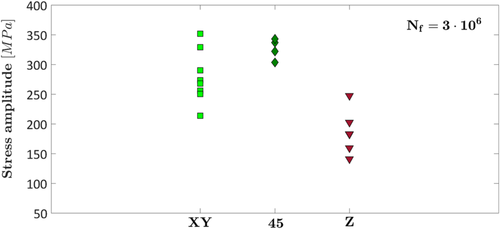
According to Figure 9, the specimens built in the Z direction show the smallest fatigue response, in agreement with the analysis carried out by Pellizzari et al.34 As discussed for the experimental results obtained in Le et al.28 in Section 3.1, the difference between the fatigue response of specimens produced in the XY direction and at 45° is not significant (p value of 7.1%), but a trend between the building orientation can be qualitatively inferred from Figure 9 and can be confirmed by considering all the experimental failures in an ANOVA with the factor “building orientation.” In this case, the p value reduces to 0, proving the dependency of the fatigue strength on the building direction. However, as highlighted by the authors, additional analyses with a larger number of experimental data should be carried out.
3.5 Stainless steel
The influence of porosities and roughness on the fatigue response of a 316L stainless steel was investigated in Solberg et al.35 Fatigue tests were carried out on as-built hourglass specimens produced with an SLM process and printed in the Z direction. The fatigue tests were carried out up to Nf = 2 · 106 in load control and at a stress ratio R = 0.1.
Figure 10A plots the experimental dataset in an SN plot, which shows that a transition between internal and surface failures exists and that the two failure modes are characterized by a different slope. Therefore, the fatigue life has been modeled by considering two failure modes and a transition stress (Equation 1 and Paolino et al.22). The estimated median, 10%, and 90% PSN curves are also shown in Figure 10A. In Figure 10B, the pdf of the transition stress is shown: The value of the transition stress found in Solberg et al.35 is also reported.
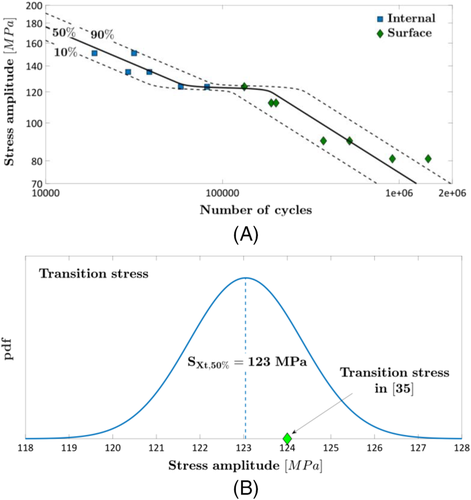
According to Figure 10A, a duplex model is appropriate to model the fatigue life for the investigated 316L stainless steel, with the transition stress properly discriminating between the two failure modes. This is confirmed by analyzing Figure 10B: The value of the transition stress in Solberg et al,35 equal to 124 MPa, is within the pdf for the transition stress estimated with the model in Equation 1. The duplex model in Figure 10B can be therefore reliably used to shift the experimental failures to the desired reference number of cycles.
3.6 Inconel
Yang et al.36 investigated the fatigue response of a Nickel alloy Inconel IN718 in the HCF and in the VHCF region. Fully reversed ultrasonic fatigue tests up to 109 cycles were carried out on hourglass specimens produced in the Z direction. The specimen shape was obtained through a machining process of as-built bars, followed by a mechanical polishing along the axial direction of the specimens. According to Yang et al,36 two different failure modes were experimentally found: failures from surface defects in the HCF region and failures from internal defects in the VHCF region, both characterized by a different slope in a traditional SN plot and separated by a transition stress.
The fatigue life was therefore modeled by considering two different slopes for the two failure modes and a transition stress (model “two failure modes and transition stress” in Paolino et al.22). The experimental data and the estimated median, 90%, and 10% PSN curves are shown in Figure 11A. In Figure 11B, the pdf of the transition stress is shown: The range of the transition stress found in Tang and Pistorius32 is also reported. Figure 11C compares the pdf of the fatigue life at a stress amplitude of 500 MPa to highlight the presence of a transition stress between the two failure modes. In particular, the pdfs are obtained by considering separately the experimental failures from surface defects and the experimental failures for internal defects (i.e., different linear models for the surface failures and for the internal failures).
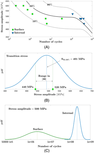
According to Figure 11A, the model for the PSN curves is in agreement with the experimental data, with the median curve subdividing the experimental failures almost equally: six failures are above the median curve, whereas seven failures are below. Indeed, if two failure modes are found experimentally, the median curve must equally subdivide the whole experimental dataset, regardless of the failure mode (i.e., it should not necessarily equally subdivide surface failures and internal failures data). The transition stress, as well as the entire dataset, is characterized by a large scatter, and this is mainly due to the small number of experimental failures in this region. A second reason is also that the stress amplitude range for the surface failures and the internal failures partially overlaps, differently from the experimental dataset in Figure 10 where stress ranges for the two failure modes are clearly distinct. Figure 11A confirms that a model involving a transition stress between the two failure modes is more appropriate to describe the fatigue life in the HCF and in the VHCF region of the tested Inconel IN718. The model can be validated by considering Figure 11B: Indeed, the range for the transition stress in Yang et al.36 is within the pdf estimated with Equation 1. Moreover, Figure 11C further confirms that surface and internal defects originate fatigue failures characterized by significantly different fatigue lives (the median value is equal to 2.1 · 106 and 2.15 · 108 cycles for the surface and internal failures, respectively) and that a transition stress should be considered to properly model the fatigue response of the tested IN718 and to discriminate between the HCF and the VHCF region.
4 DISCUSSION
This section summarizes the results of the analyses carried out in the paper, and the potentialities of the proposed methodology are discussed. Table 2 reports the experimental results obtained in the paper by applying the statistical method described in Section 2, which are generally in agreement with those obtained in the original paper.
| Paper | Material | Test up to | Process | Main results |
|---|---|---|---|---|
| Le et al.28 | 23 ELI TA6V alloy | 2 · 106 | SLM |
|
| Masuo et al.29 | Ti6Al4V | 107 | DMLS and EBM |
|
| Günther et al.30 | Ti6Al4V | 3 · 109 | SLM and EBM |
|
| Qian et al.31 | AlSi10Mg | 109 | SLM |
|
| Tang and Pistorius32 | AlSi10Mg | Test at 80 and 100 MPa | SLM |
|
| Meneghetti et al.33 | Maraging steel | 2 · 106 | SLM |
|
| Pellizzari et al.34 | H13 steel | 2 · 106 | SLM |
|
| Solberg et al.35 | 316L steel | 2 · 106 | SLM |
|
| Yang et al.36 | Inconel IN718 | 109 | SLM |
|
According to Table 2, a large number of papers focus on the effect of building direction, which is found to strongly affect the HCF as well as the VHCF response. In general, the fatigue response for XY specimens is found to be enhanced with respect to that of Z specimens, and no significant difference is found for specimens built in XY direction and at 45°. Only in one case,33 the fatigue response of Z specimens is found to be enhanced in the HCF region, as the influence of the building orientation strength is found to be a function of the number of cycles to failure. Moreover, the SLM process is proved to manufacture specimens characterized by a fatigue strength larger than that of specimens produced through the EBM process29, 30; in particular, in Günther et al,30 it is found that a HIP process on specimens produced through SLM permits to strongly enhance the fatigue response.
The influence of hatch spacing is investigated in Tang and Pistorius,32 and it is found that smaller hatch spacing (0.16 mm) permits to enhance the fatigue response. In all the investigated cases, the statistical methodology described in Section 2 has been shown to be in agreement with the analyses and the results obtained in the original papers. Moreover, it is shown that the possibility to shift all the data at a reference number of cycles to failure (or at a reference stress amplitude) permits to more properly take into account the intrinsic data scatter and to apply statistical methodologies (e.g., ANOVA or hypothesis tests) whose results can strengthen the analyses. The use of the marginal curves, furthermore, permits to model the dependency between the fatigue life and the defect size, which is, in turn, affected by the manufacturing parameters, as highlighted in the paper.
Finally, in two papers,35, 36 two failure modes are found: in Solberg et al,35 internal failures are found to occur at high-stress amplitudes in the HCF region, whereas surface failures are found in the HCF region at lower stress amplitude. In Yang et al,36 surface failures are found in the HCF region, whereas internal failures are found in the VHCF region. In both cases, a transition stress between the two failure modes is found. Even in this case, the general model in Equation 1 is found to be in agreement with the experimental data, with the estimated transition stress very close to the value and the range found in the original papers.35, 36 In addition, thanks to the proposed methodology, also the scatter associated to the transition stress between the two failure modes can be assessed, permitting for more reliable analyses. Indeed, a model that does not take into account the transition stress and its scatter could lead to a wrong interpretation of the results.
To conclude, all these examples proved the validity of the proposed statistical methodology, which can be safely used to compare experimental data obtained at different stress amplitudes, by taking into account the influence of defects, which is well-known to be the main responsible for fatigue failures in AM components.
5 CONCLUSIONS
The fatigue response of parts produced through AM processes is strongly affected by the defect population and, in particular, by the distribution of the defect size. The models considered for assessing the fatigue response of AM parts and the influence of investigated factors on the fatigue response (e.g., manufacturing process) should therefore necessarily take into account the defect size and its distribution. However, due to the limited number of experimental data available, the analysis of the fatigue results can be difficult, and the interpretation of the results can be misleading, especially if the data are obtained at different stress levels, and for each level, the number of data is small.
The present paper proposed a statistical methodology for the analysis of the results of fatigue tests performed on AM specimens. The method is based on a statistical model for the fatigue life capable of taking into account the dependency between the fatigue life and the defect size distribution. Starting from the estimation of the PSN curves, with the proposed method, all the experimental failures can be gathered at a reference number of cycles to failure or at a reference stress amplitude for a more reliable comparison. In this way, the scatter associated with the experimental failures can be taken into account and more reliably assessed.
The proposed methodology was validated on literature datasets and proved to be effective. The results obtained were found to be in sound agreement with those reported in the papers from which the datasets were taken. The statistical analyses confirmed the results found in the original papers: The analyses were carried out by applying also the ANOVA, giving more strength to the results. For the experimental data characterized by two failure modes and a transition stress, the proposed general model was also applied, proving its adaptability.
To conclude, a simple and effective methodology was proposed for the accurate assessment of the fatigue response for AM parts. The methodology can be effectively employed to soundly analyze the results of fatigue tests performed on AM parts and to extract the maximum information available from the experimental tests.
ACKNOWLEDGMENTS
Guian Qian acknowledges the support by the National Natural Science Foundation of China (Nos.11932020, 12072345, and 11872364) and CAS Pioneer Hundred Talents Program.
AUTHOR CONTRIBUTIONS
A. Tridello retrieved the literature data, analyzed the data, and wrote the paper; C. Boursier Niutta retrieved the data and contributed to write the paper; F. Berto and G. Qian retrieved the data, revised the manuscript, and supervised the work; D. S Paolino suggested the statistical model, revised the manuscript, and supervised the work.
NOMENCLATURE
-

-
- equivalent critical defect size
-

-
- cumulative distribution function of the transition stress
-


-
- conditional fatigue life
-
- FY|HCF(y; x)
-
- marginal cumulative distribution function of the fatigue life in HCF
-
- FY|VHCF(y; x)
-
- marginal cumulative distribution function of the fatigue life in VHCF
-
- FY(y; x)
-
- cumulative distribution function of the fatigue life
-
- Nf
-
- number of cycles to failure
-
- Nref
-
- reference number of cycles to failure
-
 , cth,g, αth,g
 -
- constant coefficients of the fatigue limit
-
- cY,H , mY,H, nY,H, cY,V, mY,V, nY,V
-
- parameters of the cdf of the fatigue life
-

-
- truncated pdf of the largest extreme value distribution (LEVD)
-
- sa
-
- stress amplitude
-
- sref
-
- reference stress amplitude
-

-
- mean of the fatigue limit
-
 ,
,

-
- mean and standard deviation of the transition fatigue strength
-


-
- mean of the fatigue life distribution
-

-
- standard deviation of the fatigue limit
-
- σY,V , σY,H
-
- standard deviation of the fatigue life
-
- cdf
-
- cumulative distribution function
-
- pdf
-
- probability density function
-
- PSN
-
- probabilistic S–N curve
-
- R
-
- stress ratio
-
- Y =
-
- log10(Nf).
-
- x =
-
- log10(sa).
-
- Φ(·)
-
- cdf of a standardized Normal distribution
Open Research
DATA AVAILABILITY STATEMENT
Data sharing is not applicable—no new data generated.


