Comparing temporal dynamics of compositional reorganization in long-term studies of birds and fish
Abstract
The composition of ecological assemblages has changed rapidly over the past century. Compositional reorganization rates are high relative to rates of alpha diversity change, creating an urgent need to understand how this compositional reorganization is progressing. We developed a quantitative framework for comparing temporal trajectories of compositional reorganization and applied it to two long-term bird and marine fish datasets. We then evaluated how the number and magnitude of short-term changes relate to overall rates of change. We found varied trajectories of turnover across birds and fish, with linear directional change predominating in birds and non-directional change more common in fish. The number of changes away from the baseline was a more consistent correlate of the overall rate of change than the magnitude of such changes, but large unreversed changes were found in both fish and birds, as were time series with accelerating compositional change. Compositional reorganization is progressing through a complex mix of temporal trajectories, including both threshold-like behaviour and the accumulation of repeated, linear change.
INTRODUCTION
The rapid compositional reorganization of ecological assemblages, rather than consistent loss of species, is a common pattern of Anthropocene biodiversity change (Blowes et al., 2019; Dornelas et al., 2014; Hillebrand et al., 2018; McGill et al., 2015). There is an urgent need for robust and meaningful methods of quantifying this temporal beta diversity, and understanding how the reorganization of ecological assemblages is progressing (Magurran et al., 2019). An important component of this research agenda is understanding the trajectories of compositional change.
Temporal trajectories of assemblage composition, reflected in temporal beta diversity, can yield important information to inform predictions of future change (Magurran & Henderson, 2010). Linear models are commonly used to characterize long-term biodiversity change and have potential to inform future scenarios, but the existence of non-linear, abrupt step changes in composition is a major obstacle (Dornelas et al., 2013). Such step changes have been documented in lake plankton, Caribbean coral reefs and pest outbreaks (Carpenter et al., 1999; Connell & Sousa, 1983; Hughes, 1994), and may have long-lasting consequences. Yet, the prevalence of these abrupt temporal shifts in ecosystems remains a matter of debate (e.g. Hillebrand et al., 2020; Montoya et al., 2018) and may depend on the environment and organism of interest.
We might expect that ecological context and choice of study organism should play an important role in determining how compositional reorganization progresses. Spatial beta diversity patterns vary across study organisms and latitudes (e.g. Soininen et al., 2007; Soininen et al., 2017), and the differences in dispersal, trophic structure and life-history characteristics which contribute to these differences are likely to impact on temporal beta diversity too. Existing cross-realm comparisons of temporal beta diversity (e.g. Blowes et al., 2019) have highlighted that marine assemblages often have higher rates of temporal turnover than terrestrial ones, but beyond this, the differences in compositional reorganization trajectories between ecosystems have yet to be explored.
Because of the availability of long-term community data, and their ecological importance as major groups of marine and terrestrial vertebrates, we investigated these differences using two exceptional studies of fish and birds from the BioTIME database (Dornelas et al., 2018): the North American Breeding Bird Survey (BBS) (USGS Patuxent Wildlife Research Center, 2014; Pardieck et al., 2015) and the ICES North Sea International Bottom Trawl survey of commercial marine fishes (NS-IBTS) (International Council for the Exploration of the Sea, 2010). We use these data sets to address three major questions about the progression of modern compositional reorganization. Firstly, how do overall temporal trajectories of compositional reorganization vary across birds and fish? Secondly, is compositional reorganization accelerating? And thirdly, is compositional reorganization progressing through repeated, gradual changes or through large, unreversed step changes?
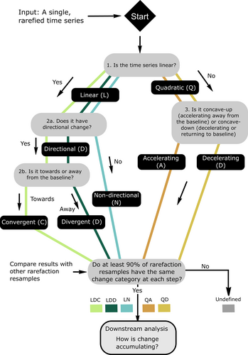
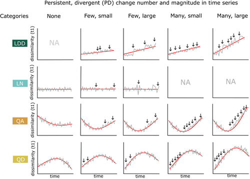
To answer these questions, we develop and apply a comparative framework for evaluating temporal trajectories of compositional reorganization (Figures 1 and 2). Our framework is: (1) quantitative; not based on subjective differences between categories of change; (2) specific; the distinctions between categories are based on specific characteristics of the time series; (3) multifaceted; the framework considers multiple attributes of temporal beta diversity; (4) intuitive; the different change categories are based on attributes of compositional reorganization which are of primary concern in the Anthropocene. Understanding the variation in temporal turnover trajectories and the relative roles of gradualistic and abrupt change across ecological contexts will help to develop frameworks for the detection and prediction of compositional change in ecological assemblages.
METHODS
General explanation of the taxonomy of turnover
A widely used approach to measuring change in assemblage composition is to use (dis)similarity metrics or multivariate methods to summarize compositional change, and then evaluate its temporal trajectory with statistical approaches including linear models (Dornelas et al., 2014), GAMs (e.g. Pandolfi et al., 2020), or breakpoint analyses (Nogué et al., 2021; Toms & Lesperance, 2003). Methods for visualizing and comparing compositional change trajectories are often focused on addressing particular research questions or data types, which inform the focal aspects of compositional change and the way they are quantified (De Cáceres et al., 2019; Matthews et al., 2013). Our framework, which we call a ‘taxonomy of turnover’, is tailored to highlight the temporal dynamics of compositional reorganization over the relatively short timescales of observational ecological time series.
The taxonomy of turnover is based on the characteristics of models fit to a time series of Jaccard dissimilarities to the composition in the first year of the time series (the baseline year). We chose this method for measuring compositional change in order to capture the temporal dynamics of rapid reorganization highlighted by earlier studies on assemblage turnover (Dornelas et al., 2014). Dissimilarities can also be calculated by comparing the assemblage within a moving window of years to a baseline window of years; this does not substantially change the results (SM2).
Methodological details of the taxonomy of turnover
We classified turnover trajectories by applying a series of quantitative tests (Figure 1), assigning each time series to a category based on the outcomes. Each category takes the form of a string of letters, each denoting the result of a test. These tests ask: (1) Is compositional reorganization happening linearly (at a constant rate) or non-linearly (accelerating or decelerating)? (L = linear, Q = quadratic). (2a) For linear time series, does the assemblage show directional compositional change? (D = Directional, N = Non-directional); (2b) for linear time series, if there is directional change, is it towards the baseline, or away from the baseline? (C = convergent change, towards the baseline; D = divergent change, away from the baseline); (3) for quadratic time series, is the rate of compositional reorganization accelerating or decelerating? (D = decelerating; A = accelerating). For example, an assemblage in the LDC category has linear, directional, convergent change. However, directional linear trends can emerge either through repeated small changes or through smoothing of larger step changes, which could yield similar overall directional trends but which imply differences in the dynamics which generate those trends. We examined linear time series more closely in a downstream analysis, which evaluates whether linear trends in time series have emerged through gradualistic or abrupt changes (see below).
To decide whether compositional reorganization is progressing linearly or non-linearly (test 1), we used the assemblage in year 1 of the time series as the baseline, and calculated the Jaccard dissimilarity of the assemblage in all subsequent years to that baseline, constructing a time series of dissimilarities. To decide whether each time series had a linear or non-linear trend, we fit a linear model to the time series using OLS regression, and a quadratic polynomial model, in each case using the years of the time series as the predictor variable and the dissimilarities as the response. The model with the lower Bayesian information criterion (BIC) value was selected; using AIC for model selection does not substantially change the results (SM3). A caveat of our approach is that we have selected either a quadratic or a linear model for each time series for classification; we do not claim that either model is the best choice to reflect the shape of all time series in our study.
For linear time series, we also addressed whether there was a significant directional trend (test 2a) and whether the trend was towards or away from the baseline (test 2b). To do this, we created a null model with no directional trend by randomizing the sequence of abundances for each species 100 times, recalculating the dissimilarity time series relative to the baseline composition and fitting a linear model to each randomized time series. If the gradient of the linear model fit to the observed assemblage time series was more than two standard deviations from the mean gradient of the 100 randomized time series, and had p < 0.05, we considered the time series to have a directional compositional gradient. Directional time series with positive gradients (where the assemblage is becoming more dissimilar to the baseline through time) were called ‘Directional divergent’, while those with negative gradients were called ‘Directional convergent’.
For time series where a quadratic polynomial was the selected model, we evaluated whether the model was concave-up (i.e. accelerating away from the baseline) or concave-down (i.e. decelerating or recovering towards the baseline) (test 3). To do this, we evaluated the second derivative of the quadratic function, which is >0 where change in assemblage composition is accelerating away from the baseline (a concave-up function) and <0 when change in assemblage composition is slowing, or where the assemblage is recovering towards the baseline (a concave-down function) (Studeny et al., 2013).
Because sample-based rarefaction results in different trajectories between rarefaction resamples of the same time series, we also compared the results of each test across rarefaction resamples, requiring 90% of resamples to agree before the results of a particular test were accepted as part of the classification for a time series. In some cases, there was 90% agreement on the first test (model selection) for the time series, but 90% agreement was not achieved on any subsequent test; this results in partial classification, where time series are assigned to, for example, class ‘L' (linear) or class ‘Q' (quadratic).
Ecological assemblage time-series data
We applied this classification scheme to data sets from the BioTIME database of assemblage time series (Dornelas et al., 2018). We selected two long-term and large-extent studies from the database: the North American Breeding Bird Survey (BBS; henceforth ‘birds’) (USGS Patuxent Wildlife Research Center, 2014; Pardieck et al., 2015) and ICES North Sea International Bottom Trawl Surveys (NS-IBTS; henceforth ‘fish’) (International Council for the Exploration of the Sea, 2010). These two studies were selected because they allow trajectories of compositional reorganization to be examined across marine and terrestrial realms, with focus on birds and fish allowing greater ecological interpretability than including the full range of taxonomic groups in the BioTIME database. To standardize the spatial scale of analysis, we assigned the data from each study to 96-km2 grid cells, following the method of Blowes et al. (2019), and treated the assemblage data within each cell of the grid as a distinct time series. Of these gridded data, we analysed only the time series with at least 20 years of sampling. We controlled for the effect of sampling effort using sample-based rarefaction on each time series which passed this filter to the smallest number of samples in any given year, repeating this process 100 times (see SM1). Because sampling was generally even in the BBS, rarefaction typically gave identical resamples within time series for this data set; more variable sampling in the NS-IBTS created greater differences between rarefaction resamples.
Background information on fish and bird studies
The BBS began in 1966 as a long-term observational programme aimed at monitoring bird population trends in North America (Robbins et al., 1986). Bird populations are monitored using roadside surveys, where observers drive a consistent route, 0.5 h before sunrise on one morning per year during breeding season (ranging from May to July depending on location). Along the route, observers make 50 stops, 0.8 km apart and record for 3 min the total number of each bird species heard, and birds seen within 400 m of the stop (Robbins et al., 1986). This study uses BBS data spanning from 1978 to 2007, comprising 699,392 records of 385 bird species.
The NS-IBTS is an annual survey aimed at collecting data for assessment of fish stocks and monitoring ecological change (ICES, 2020). Fish assemblages are sampled on a fixed grid, with rectangular cells of approximately 1 degree of longitude and 0.5 degrees of latitude. Each rectangle is sampled with two hauls, generally conducted by two different vessels. These vessels may trawl at any position within a rectangle as long as the two hauls are at least 10 nautical miles (approximately 18.5 km) apart. This study uses NS-IBTS data from the years 1965–2011, comprising 347,445 records of 271 taxa.
Downstream analysis: ‘How is long-term directional change generated?’
Long-term directional change emerges from shorter term shifts away from the baseline composition, from which the assemblage does not completely recover. We term these ‘persistent divergent’ (PD) changes. Time series with different overall trajectories are expected to differ in the number and magnitude of PD changes. As well as evaluating whether compositional reorganization is accelerating, we also wanted to determine whether directional changes were occurring gradually through many small PD changes, or abruptly through few large ones (Figure 2). To address this question, we calculated the number and magnitude of PD changes in each time series. We calculated the first differences of all the dissimilarities in each rarefaction run of an assemblage time series, generating a time series of the sign and magnitude of compositional changes relative to the baseline in each time step. To evaluate which changes had a lasting impact on the composition of the assemblage, we calculated the cumulative sum of each divergent change (away from the baseline), and all subsequent changes. If the cumulative sum reaches zero, then at some point, the assemblage recovers from the initial divergent change, and it does not contribute to overall directional change in the time series. If the cumulative sum never reaches zero, then the initial divergent change has persisted. We considered only the persistence of changes away from the baseline, not towards it.
We selected standardized time intervals of 1 and 5 years across which change was measured, so that the magnitude of change occurring across an interval is a proxy for the rate. These intervals were selected because we wanted to capture the shortest term changes (1 year) without overlooking changes which might take years to accumulate, such as gradual responses to disturbance. We measured the changes which led to the Jaccard dissimilarity to baseline in a given year by counting back by the specified number of time steps (1 or 5). Time series do not always have samples in every year; we ignored divergent changes which had occurred over sampling gaps longer than our stated 1- or 5-year interval.
The magnitude of change alone is not sufficient to determine whether it is ‘abrupt’ in the context of a specific ecological time series. Ecological assemblages have varying degrees of compositional variability over time, with marine time series tending to have higher temporal variability than terrestrial ones (Blowes et al., 2019). To evaluate whether the maximum PD changes in a time series were unusually large, we also checked whether they fell within the top quartile of change magnitudes within each time series.
This process was repeated for each of the rarefied dissimilarity time series from each assemblage, and we calculated the maximum magnitude of PD change across all 100 rarefaction resamples. The maximum PD change magnitude was chosen in preference to an average, to ensure that the analysis did not miss large PD changes occurring within time series. We also calculated the mean number of PD changes occurring across the resamples, and the mean slope for linear time series.
All analyses were run in R version 4.1.3 (R Core Team, 2022); Jaccard dissimilarity was calculated using the function vegdist() in R package ‘vegan’ version 2.6–2. (Oksanen et al., 2022) and plots were made using ggplot2 (Wickham, 2016).
RESULTS
After gridding and filtering to retain only time series containing at least 20 years of data, the BBS bird data set contained 439 time series, ranging in length from 28 to 30 years. The NS-IBTS marine fish data set contained 169 time series, with between 20 and 38 years of data (SM4).
Prevalence of change categories
Linear and non-linear temporal trajectories of compositional reorganization were common in both studies (Figure 3). In fish, 54 time series (12.4%) showed non-linear temporal trajectories, of which 11 were decelerating or returning towards the baseline (category QD) and 10 were accelerating away from the baseline (category QA). In birds, 111 (25.3%) of time series had non-linear trajectories, of which 82 were decelerating or returning towards the baseline and 29 were accelerating away from the baseline. Around 30% of fish time series were assigned to category ‘Undefined’; in these time series, there was less than 90% agreement between rarefaction resamples on whether the trend was linear or quadratic. This ‘Undefined’ category was more common in fish than in birds because uneven sampling in the fish time series led to greater differences between rarefaction resamples after sample-based rarefaction.
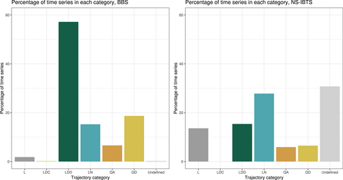
Time series showing linear change towards the baseline (category LDC) were very rare; the bird data set contained only one time series which showed this pattern, and the fish data set contained none. This type of change probably emerged as a result of the assemblage recovering linearly from an initial perturbation early on in the time series (Dornelas et al., 2014a). Across both studies, non-directional linear change (category LN) and directional linear change away from the baseline composition (LDD) were both common, but directional linear change was much more common than non-directional linear change in birds (57.2% for LDD compared with 16.3% for LN), while non-directional linear change was more common than directional divergent linear change in fish (15.4% for LDD compared with 27.8% for LN).
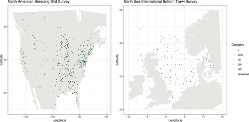
Both studies also contained a minority of linear time series with no robust directionality category (category L); 13.6% for fish and 1.8% for birds. Although sampling is very even in the bird study, a time series can still be assigned to category L where the test of directionality returns differing results among 100 identical rarefaction resamples. Both data sets also contained time series where fewer than 90% of the rarefaction resamples returned the same result for each test, so no change category was assigned. This was much more common in fish than birds, as sampling was less even in the fish time series, and consequently, there was more variability between rarefaction resamples. There was no clear pattern in the spatial distribution of different trajectories of compositional reorganization (Figure 4).
Magnitude and number of PD changes in time series with different trajectories
In fish, time series with different overall trajectories had significant differences in the maximum magnitude of PD changes, whether these changes were measured over 1 or 5 years (Kruskal–Wallis chi-squared = 14.8, p = 0.01 with changes measured over 1 year; Kruskal–Wallis chi-squared = 16, p < 0.01 with changes measured over 5 years) (Figure 5). The mean number of PD changes was not significantly different between trajectories when changes were measured over 1 year (Kruskal–Wallis chi-squared = 9.14, p = 0.10) or 5 years (Kruskal–Wallis chi-squared = 7.95, p = 0.16).
In birds, there were significant differences in the number and magnitude of PD changes across change trajectories, regardless of whether these changes were measured across 1 year or 5 (Figure 5). The number of PD changes differed significantly across change categories (Kruskal–Wallis chi-squared = 72, p = 2e-13 when change was measured across 1 year, or Kruskal–Wallis chi-squared = 92.72, p < 0.01 when change was measured across 5 years). Significant differences in the number of 1-year PD changes were between LDD and LN, QD and QA time series (p < 0.01, p < 0.01 and p = 0.0123, respectively), between LN and both QD and QA time series (p < 0.01 in both cases), and between QD and QA time series (p < 0.01). The pattern was similar when changes are measured across 5 years.
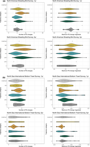
PD change magnitudes also differed significantly between change categories in birds. There were significant differences in the magnitude of PD changes, when PD changes were measured across 1 year (Kruskal–Wallis chi-squared = 25, p = 3e-04), with a Dunn's test showing significant differences between LDD and LN time series (p < 0.01), LDD and QA (p = 0.0183) and LN and QD (p < 0.01). There were also significant differences when changes were measured across 5 years (Kruskal–Wallis chi-squared = 17.7, p < 0.01); between LDD and LN (p = 0.01), LDD and QD (p < 0.01), LN and QA (p < 0.01) and QA and QD (p < 0.01).
Contribution of gradual and abrupt change to linear directional change
An assemblage time series might follow a ‘linear’ trajectory because it has undergone many changes away from the baseline, or because it has undergone a smaller number of step changes, where the assemblage might be stable for several years between steps. To distinguish these two scenarios, we plotted the mean number, and maximum magnitude of PD changes against the mean slope of each linear trajectory, for the two studies (Figure 6a,b). Whether large or small in absolute terms, the maximum PD change magnitudes within time series mostly fall within the top quartile of change magnitudes within their time series.
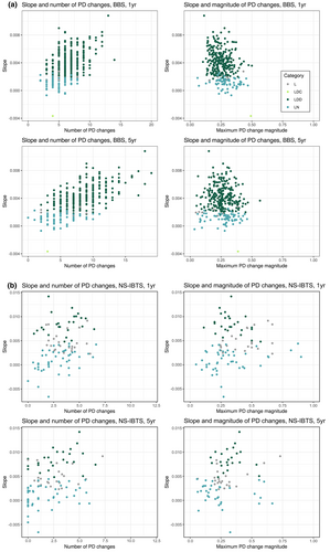
In birds, linear time series showed a weak negative correlation between slope and maximum PD change magnitude measured across 1-year intervals (Kendall's tau = −0.19, p < 0.01) or across 5-year intervals (Kendall's tau = −0.08, p = 0.04). There was a moderate positive correlation between the number of PD changes and the slope when PD changes were measured across 1-year intervals (Kendall's tau = 0.36, p = <0.01), which strengthened when PD changes were measured over 5-year intervals (Kendall's tau = 0.48, p < 0.01).
In fish, there was a weak positive correlation between the slope of linear time series and the maximum PD change magnitude measured across 1-year or 5-year intervals (Kendall's tau = 0.16, p = 0.03; Kendall's tau = 0.20, p < 0.01, respectively). There was also a weak positive correlation between the slope and the number of PD changes, whether a 1-year or 5-year measurement interval was used (Kendall's tau = 0.23, p < 0.01; Kendall's tau = 0.24, p < 0.01, respectively).
Correlations between the number and magnitude of PD changes, and the duration, number of years sampled and starting year of each time series are examined in SM5 and SM6. In fish, the number of PD changes in a time series correlated weakly but positively with initial species richness when PD changes were measured over 5 years (Kendall's tau = 0.14; p = 0.06 for 1-year PD changes; Kendall's tau = 0.21, p < 0.01 for 5-year PD changes). The magnitude of PD changes correlated weakly with initial species richness, but only when PD changes were measured across a 5-year lag (Kendall's tau = 0.12, p = 0.09 for 1-year PD changes; tau = 0.24, p < 0.01 for 5-year PD changes). In birds, there was no correlation between number of PD changes and initial species richness (Kendall's tau = 0.03, p = 0.41 for 1-year PD changes; Kendall's tau = 0.04, p = 0.33 for 5-year PD changes), and the magnitude of PD changes correlated negatively with species richness (Kendall's tau = −0.23, p < 0.01 for 1-year PD changes; tau = −0.26, p < 0.01 for 5-year PD changes).
DISCUSSION
Variation in overall temporal trajectories of compositional reorganization in birds and fish
Our results underline that directional change in assemblage composition is common, as observed by, for example, Dornelas et al. (2014), but there are striking differences in the prevalence of different temporal trajectories across the two studies. Trajectories showing no significant directional change are proportionally more common in fish, while linear, directional change away from the baseline is much more common in birds.
These differences probably result from a combination of differences between the ecological characteristics of birds and fish, and the distinctive pressures which North American birds and North Sea fish have experienced. Intrinsic differences between marine and terrestrial ecologies are well-documented: Barriers to dispersal are rarer in marine environments (May, 1994), the main marine primary producers are smaller, shorter lived and more sensitive to short-term environmental change than terrestrial ones, habitat associations and trophic characteristics are more variable within fish species than bird species, and fish tend to produce very large numbers of eggs while birds produce just a few (Webb et al., 2011). High variability in primary production, easy dispersal and low local persistence in marine environments would all contribute to reducing the prevalence of directional assemblage change in fish, compared with birds. Over a given timescale, significant compositional change may also be more difficult to detect in assemblages with higher compositional variability, and local-scale compositional reorganization is less likely in an environment where inward dispersal can quickly replace species which are locally extirpated.
Distinct pressures on biodiversity may also create differences in compositional reorganization between fish and birds. Data collection routes used in the BBS have experienced increases in traffic volume and development, as well as climatic change (Sauer et al., 2017). More generally, terrestrial ecosystems have experienced considerable biodiversity change in recent decades, for example, due to land use change (Bowler et al., 2020). Marine fish assemblages in the North Sea face pressures related to climate change (Engelhard et al., 2014), overharvesting (Daan et al., 2005), disruption to benthic habitats due to repeated trawling (Couce et al., 2020) and climate-driven compositional change (Antão et al., 2020). There is no obvious large-scale spatial pattern in where different trajectories of assemblage change occur in the two studies, suggesting that small-scale drivers help to determine how compositional reorganization progresses within assemblages.
Acceleration of compositional reorganization
Compositional reorganization is progressing non-linearly in a substantial minority of time series from both studies. Assemblages with concave-up non-linear trajectories (QA) are potentially showing accelerating rates of compositional change (Figure 3). In practice, time series where the temporal trajectory of assemblage composition forms a parabola are rare, but accelerating compositional change is consistent with earlier results (Dornelas et al., 2019).
Non-linear, convex-up trajectories (QD) suggest either a decline in the rate of compositional reorganization or recovery towards the baseline. In both fish and birds, PD change occurs at a wide range of frequencies in QD time series; a low number of PD changes could suggest that the assemblage is recovering towards its baseline composition, as early shifts away from the baseline are cancelled out later on. QD time series with large numbers of PD changes may reflect either recovery towards the end of the time series, or the stabilization of the assemblage at a new composition. Distinguishing between these scenarios without further monitoring would require local-scale information on the drivers of compositional change and their likely reversibility. Comparison of fish and bird surveys suggests that this non-linear, recovering or stabilizing trajectory is accompanied by more PD changes in birds than in fish (Figures 3 and 5).
Progression of compositional reorganization through repeated, gradual change or exceptional, large changes
Linear trends in time series from the bird and fish surveys emerge through different dynamics. In birds, rates of linear change within time series are not positively correlated with the maximum magnitude of PD changes within those time series. Instead, there is a positive correlation with the number of PD changes within time series, suggesting that linear trends away from the baseline are generally emerging through repeated shifts, rather than through exceptional, catastrophic step changes.
The fish data set presents a more complex picture. Overall rates of change correlate positively with both the number and magnitude of PD changes, though these correlations are weak. Directional change in assemblage composition in fish is emerging due to both repeated shifts and through threshold-like behaviour. These changes may take several years to emerge, and the presence of large PD changes in time series which lack a significant directional trend (LN time series, Figure 5b) suggests that high variability in fish assemblages could have masked the impact of such directional change.
Wider implications for the dynamics of compositional reorganization
In the fish and bird datasets analysed here, compositional reorganization followed a variety of different temporal trajectories, driven to varying extents by patterns of gradual and abrupt change. Abrupt changes, which can take some years to emerge, play an important role in determining the overall rate and trajectory of compositional change, though their importance is context-specific. We find that repeated (gradual) change plays a more consistent role than large rapid change events in determining the trajectories of change which emerge, and rates of linear change. The paradigm of biodiversity change through catastrophic phase shifts (e.g. Scheffer et al., 2001; Scheffer & Van Nes, 2007) does not reflect the most common trajectories of compositional reorganization in our study, an observation also made by Hillebrand et al. (2020). Compared with other biodiversity metrics, assemblage composition is relatively slow to recover from pulse disturbances (Hillebrand & Kunze, 2020), and this may contribute to the tendency for compositional changes to accumulate over time.
This does not mean that critical transitions do not occur; they are a well-documented feature of the dynamics of some ecosystems (e.g. Carpenter et al., 1999; Hughes, 1994; Isbell et al., 2013). The minority of fish and bird time series which show accelerating compositional change raise the question of whether non-linear change will become more common in future. Critical ecological changes are not always fast: the recorded coral–macroalgal regime shift in Caribbean coral reefs developed over decades (Hughes, 1994), as did reported phase shifts in coral reef composition (Aronson et al., 2004). A longer term perspective on the dynamics of biodiversity change would improve understanding of whether patterns of biodiversity change from the past few decades will continue into the future (Davies, 2016; Hughes et al., 2013).
The importance of level of organization for understanding patterns of rapid and gradual change
Documented examples of sudden, unreversed assemblage change tend to focus on systems which respond rapidly (e.g. lake assemblages in Carpenter et al., 1999) and are often focused on relatively small numbers of species where the disease outbreaks, ecological interactions and disturbances which generate a rapid transition can be identified and modelled (e.g. Hughes, 1994; Reid et al., 2001; Weijerman et al., 2005). We might expect rapid transitions to be rarer in more species-rich assemblages, if only because the loss or gain of a single species has a proportionally smaller impact on an already species-rich assemblage. The negative correlation between species richness and magnitude of PD changes in bird time series may reflect this effect, but we found no such relationship in fish assemblages. Compositional reorganization in North Sea fish assemblages is driven by a small subset of species (Gotelli et al., 2022), and the generally lower species richness of fish assemblages in this study may make assemblage composition more responsive to the persistence of single populations.
Conservation and monitoring implications
A paradigm of biodiversity change which focuses exclusively on abrupt step changes and critical thresholds risks overlooking the repeated compositional changes which accumulate to generate most compositional turnover, and the diversity of compositional change trajectories (see also Hillebrand et al., 2020; Hughes et al., 2013; Montoya et al., 2018). One implication for the monitoring and forecasting of biodiversity change is that long-lasting changes in assemblage composition can be small in magnitude. Rather than providing a general paradigm of ecological change, the concept of directional change through unusually rapid shifts has the most utility when the temporal scale and resolution, natural variability of the system and targeted level of organization are clearly specified, rather than being a general expectation for ecological change.
Ongoing biodiversity monitoring efforts will be needed to determine whether the tendency towards gradual directional change will continue, as a gradual pattern of change in the past does not rule out abrupt change in the future (Folke et al., 2004; Holling, 1973; Scheffer et al., 2001). Further investigation is needed into the implications of widespread, rapidly accumulating changes in assemblage composition. A temporal trajectory of gradual directional change, rather than abrupt step changes, is sometimes interpreted as more readily reversible (Hughes et al., 2013), but in practice, this reversibility depends on the drivers of change and their amenability to intervention.
CONCLUSIONS
We applied a consistent, quantitative framework to classify trajectories of compositional reorganization over the past several decades in two large, long-term studies of North Sea fish and North American birds. We then asked how the number and magnitude of short-term changes have contributed to these trajectories. Compositional reorganization has followed a variety of trajectories, with linear, directional change away from the baseline more prevalent in birds than in fish. The number of changes away from the baseline is a more consistent correlate of rates of linear change in composition than the magnitude of such changes, though the persistent short-term changes tend to be in the top quartile of change magnitudes within their time series. This result suggests that most assemblages undergoing directional change either lack ecological thresholds or have been changing incrementally and may be amenable to recovery. However, large, unreversed changes have happened in some assemblages, and the continuation and expansion of ecological monitoring efforts will be critical to understanding the implications of these changes.
AUTHOR CONTRIBUTIONS
Amelia Penny, Maria Dornelas and Anne Magurran conceived this study and designed the analyses. Amelia Penny processed data, performed quantitative analyses and drafted the manuscript and figures. All authors made substantial contributions to the manuscript text and figures.
ACKNOWLEDGEMENTS
AP acknowledges funding from Leverhulme Trust grant RPG-2019-402, Darwin, Wallace, Bates and biodiversity change in the Anthropocene, awarded to AM & MD, and also thanks Faye Moyes, Inês Martins, Viviana Brambilla, Ada F. Eslava and Cher Chow for support with code and data. We thank Dr Christopher Terry (University of Oxford) for helpful feedback, and reviewers of this manuscript for their incisive and constructive comments. We also thank the collectors of data used in this study.
Open Research
DATA AVAILABILITY STATEMENT
All data supporting these results are available from the BioTIME database (https://biotime.st-andrews.ac.uk/) or from OBIS (https://obis.org/dataset/ad65221f-0539-44aa-925e-4acf62ad0c6a). Data and code required to replicate the analyses in this study are available on Zenodo at the following DOI: 10.5281/zenodo.7665559


