Random regression models to estimate genetic parameters for weights in Murrah buffaloes

Introduction

The water buffalo (Bubalus bubalis) has an important economic role in many countries, being used for meat, milk and work purposes. Therefore the genetic improvement of this species for milk production and quality has an important economic and social impact worldwide, especially in developing countries (Misra & Tyagi 2007). The interest in the species has increased because of its ability to convert tropical grass into meat or milk, good environmental adaptability and high fertility (Borghese 2005). Based on information from FAOSTAT (2015), the global production of buffalo milk and meat has shown annual growth of 3.60% and 2.56%, respectively, India being the largest producer.

Body growth is an important selection criterion in dairy animals, due to the genetic correlation with reproductive and productive traits (Vercesi Filho et al. 2007). Many studies have reported estimates of genetic parameters for weight at different ages, using single or multi-trait animal models (Malhado et al. 2012; Agudelo-Gómez et al. 2015). Random regression models (RRM) have shown the greatest efficiency for analysis of growth curves, because the weights are measured along a continuous scale (Kirkpatrick et al. 1990). Few studies of buffaloes have been conducted until now (Bolivar et al. 2013). For this reason, we performed a genetic analysis of the weights at different ages of Murrah water buffaloes, up to the age of 600 days, applying RRM.

Materials and Methods

Animal Care and Use Committee approval was not necessary for this study because the data were obtained from an existing database. We used weight data on 2322 male and female Murrah buffaloes, with measurements taken between the ages of 30 and 600 days. The animals were from a herd kept at Tapuio Farm, a participant in the dairy quality program promoted by São Paulo State University (UNESP), Jaboticabal campus. The main activity of Tapuio Farm is the production of mozzarella cheese. It covers an area of 496 hectares and is located in the municipality of Taipú, Rio Grande do Norte state (latitude S 5°33′57.13″ and longitude W 35°37′37.98″). The animals are managed in a Voisin rotational pasture system, with daily grazing in paddocks measuring 0.8 ha with Marandu grass (Brachiaria brizantha cv. Marandu) and Massai grass (Panicum maximum cv. Massai).

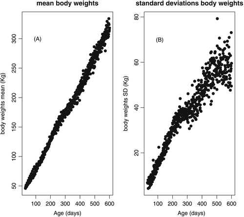
Contemporary groups (CGs) were formed by concatenation of the variables birth year, sex, birth season and weighing year, and after procedures to assure consistency: (i) elimination of CGs with fewer than 10 records; (ii) elimination of records more than 3.5 standard deviations from the mean of the CG; and (iii) elimination of animals with fewer than five weight records. The basic data and statistics are presented in Table 1, and the mean and standard deviation of weights at different ages are presented in Figure 1.

To estimate the co(variance) parameters of the weights at different ages, we employed RRM with orthogonal Legendre polynomials of third to sixth order about age at weighing. All models used included the direct genetic and animal permanent environmental effects as random effects, and contemporary group and mean population curve as fixed effects, modeled using third-order Legendre polynomials. On the farm in question, the calves are separated from the dam on the fifth lactation day (to enable use of the colostrum), after which they are fed milk artificially. For some cows the calf's presence at the beginning of milking is necessary to stimulate the glandular activity, but this contact is limited to few minutes in the day. Because of this slight maternal influence, we did not include effects of maternal origin in the model, as is usually the case in random regression studies. The RRM can be described as:

where y_ij is the weight at ith age of animal j; F is the set of fixed effects (contemporary groups); β_m are regression coefficients to model the average trajectory of the population; φ_m(t_i) is the mth Legendre polynomial according to age (t_i); φ_m(t_ij) are regression functions describing the trajectories of each individual j according to age (t_i) for the following random effects: direct genetic and animal permanent environmental effects; α_jm and δ_jm are individual random coefficients of direct genetic and animal permanent environmental effects; k_b, k_a and k_p are the order of polynomials used for the effects described in the model, and E_ij is a random error associated with each age i of animal j. The matrix representation of the model is:

where y is the vector of observations, b is the vector of fixed effects (including F and βm), a is the vector of random coefficients for direct genetic effects, p is the vector of random coefficients for animal permanent environmental effects, and X, Z and W are the corresponding incidence matrices. The model is based on the following assumptions:

where K_A and K_C are (co)variance matrices between random regression coefficients for direct genetic and animal permanent environmental effects, respectively; A is the pedigree-based numerator relationship matrix; I is an identity matrix; n is the number of animals for which records are available; ⊗ is the Kronecker product between matrices; and R is a block diagonal matrix containing residual variance. Correlations between random regression coefficients for different effects were set to zero.

The residuals were modeled considering the heterogeneity of the residual variances, through a quadratic variance function assuming a log-linear model, as described by Misztal et al. (2014). The nomenclature used in the models is Mk_ak_p, where k_a and k_p are placeholders for the order of the Legendre polynomial used to model the genetic effect and permanent environmental effect, respectively.

For the estimation of the co(variance) matrix between the random regression coefficients, we used the restricted maximum likelihood method (REML), employing the AIREMLF90 software (Misztal et al. 2014), through maximization and expectancy and average information algorithms. All told, we tested seven models with polynomials with orders varying from three to six, for both random effects considered. The models' performance was compared using the Akaike information criterion (AIC) and Bayesian (or Schwarz) information criterion (BIC), which permit comparison of non-nested models and penalize more parameterized models, such that:

where: p = number of parameters in the model; N = number of observations; and r = rank of matrix X (incidence matrix for the fixed effects). The AIC and BIC test the fit of the model considering the number of parameters and can be used to compare models with the same fixed effects but different (co)variance structures. The BIC attributes a greater penalty for additional parameters than AIC does. Smaller values of AIC and BIC are preferred (Boligon et al. 2010).

Results and Discussion

The models with a greater number of parameters presented higher values of logL. Two different models (M66 and M36) were selected using the two information criteria employed, AIC and BIC, respectively (Table 2). Regardless of the selection criterion used, for the animal permanent environmental effect the models selected were those with the largest number of parameters. This need for a higher-order polynomial to model this effect was found previously in other studies of dairy and beef cattle (Brotherstone et al. 2000; Meyer 2001). Other studies using random regression to analyze body weight in cattle (Boligon et al. 2010; Souza Júnior et al. 2010) and buffalo (Bolivar et al. 2013) have found the need for higher orders for direct genetic effects than we found.

Analysis of the eigenvalues of the two models chosen (Tables 3 and 4) for direct genetic effect showed that the change in this statistic in M66, above the third order, is small, which can indicate that an M36 model is sufficient to estimate the parameters. However, because of the discrepancy in the number of parameters in the models selected by the different criteria, we considered both in the elucidations about the variance and genetic parameters.

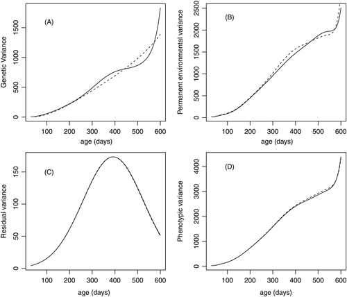
The direct genetic variances behaved similarly in the two models, with a rising trend during the animal's lifetime (Fig. 2A). This rising trend of the direct genetic variance has also been reported in studies with buffaloes in Colombia (Bolivar et al. 2013) and Nelore and Tabapuã cattle in Brazil (Albuquerque & Meyer 2001; Nobre et al. 2003; Dias et al. 2006).

Regarding the variances of the animal permanent environmental effect (Fig. 2B), there was also a tendency for increased variances with animal age, with similar curves between the models. In model M36, the variances of the animal permanent environmental effect were slightly higher from 300 to 450 days and lower from 470 to 570 days, after which age they started to increase again, more pronounced in comparison to model M66 (Fig. 2B). Increases in the animal permanent environmental variances, from birth to 600 days, have also been reported by Dias et al. (2006), Boligon et al. (2010) and Souza Júnior et al. (2010) in cattle, and by Bolivar et al. (2013) in buffaloes.

The coefficients of the quadratic variance function assuming a log-linear model used for estimation of residual variance are reported in Tables 3 and 4. The residual variance behaved similarly in the two models (Fig. 2C), where the residual variance increased until near 365 days of age, after which this statistic declined.

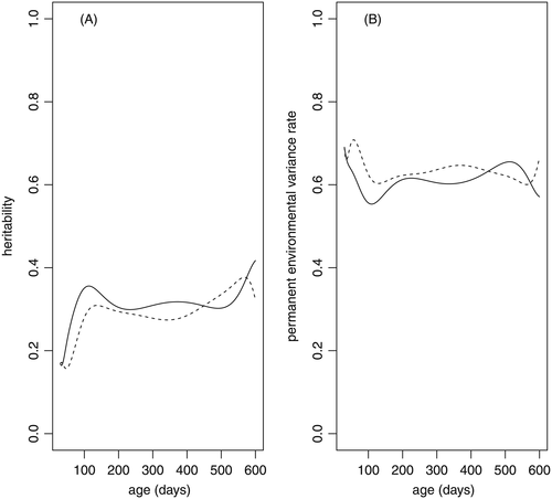
The heritability estimates for the body weights at different ages (Fig. 3A) showed similar behavior between the two models, where we can highlight a greater magnitude of the estimates in the initial phase, with subsequent stability and then a renewed increase at ages greater than 400 days. The estimates of heritability varied from 0.16 ± 0.04 (44 days) to 0.38 ± 0.04 (568 days) in model M36 and from 0.16 ± 0.05 (33 days) to 0.42 ± 0.05 (600 days) in model M66. In both models the heritability increased until near weaning (100 days of age), with values of 0.31 ± 0.03 (136 days) and 0.36 ± 0.04 (113 days) for M36 and M66, respectively.

The heritability values found were similar to those reported by Souza Júnior et al. (2010), studying Tabapuã cattle, who found values that fluctuated from 0.15 for weight at birth to 0.45 for weight at 660 days of age. However, the values observed were lower than those estimated for Nelore cattle by Boligon et al. (2010) and for Canchim cattle by Baldi et al. (2010). This lower heritability and the lower orders for direct genetic effects in relation to bovine breeds can be explained by the production system, since we studied dairy animals where the management and feeding regimen are not designed to maximize the growth.

From the estimated heritability values obtained in this study, it was possible to infer that significant genetic gains can be obtained by selecting animals for weight at different ages, which assumed values with medium to high magnitude. From these values, greater genetic differences could be observed between animals near weaning and at older ages (near 600 days). These are the phases where genetic selection will be most efficient. Since the heritability estimates in these periods are similar, the selection based on younger age becomes interesting, due to: (i) the shorter generation interval; and (ii) the small indirect genetic gain in adult weight, arising from the smaller estimated genetic correlation reported in the literature between weight at pre-weaning ages and adult weight (Baldi et al. 2010; Boligon et al. 2010).

With respect to the animal permanent environmental effect, the proportion of this effect in relation to the total variance presented estimates that ranged between 0.60 ± 0.04 (536 days) and 0.71 ± 0.03 (57 days) for model M36 and between 0.55 ± 0.04 (110 days) and 0.69 ± 0.05 (30 days) for model M66 (Fig. 3B). Lower values of these statistics were reported by Souza Júnior et al. (2010), who observed a tendency for growth from birth (0.01) to 160 days of age (0.29) followed by gentle decline to 440 days (0.23) and virtually constant values thereafter (0.24).

The estimates of direct genetic (Table 5), animal permanent environmental (Table 6) and phenotypic correlations (Table 7) showed the same pattern as reported in other studies employing the random regression method (Baldi et al. 2010; Boligon et al. 2010; Bolivar et al. 2013), in which the magnitude tends to diminish with increases in the interval between measurements, assuming the classic ‘saddle’ shape. In general, model M36 presented greater correlation values than model M66. The magnitude of the associations tended to change less with increase of the period between measurements. In buffaloes, Bolivar et al. (2013), analyzing weight values between ages of 240 and 900 days, found estimates varying from 0.71 (300 and 900 days of age) to 0.99 (240 and 270 days). A greater amplitude of values was described by Baldi et al. (2010), who estimated correlations between 0.45 and 0.97, considering weight at birth, weight at weaning, adult weight and weights at ages of 12, 18, 24 and 30 months.

Based on the results presented, considering that the direct genetic correlations between weight measurements at the various ages have large magnitude, selection for greater direct and indirect genetic gain should be done at ages that presented the highest heritability estimates (100 and 568 days). However, unlike for other bovine species, buffaloes still have not been found to present defined specialization for milk or meat production. Therefore, the way to use the body weight criterion for selection will depend on the production system.

In cattle, the genetic correlation of weight at older ages with reproductive traits has shown favorable association in males (Araujo Neto et al. 2011) and females (Mercadante et al. 2000; Berry et al. 2003; Gaviolli et al. 2012), with magnitudes having low to moderate values. This favorable association with reproductive traits means weight is an additional selection criterion that can be used in dairy production systems. However, studies of dairy cattle have verified an unfavorable association between body weight and milk production. Vercesi Filho et al. (2007), studying mestizo dairy cows, reported genetic correlation estimates of −0.59, −0.73, −0.62 and −0.67 for growth rate with milk yield, fat and protein content and duration of lactation, respectively. Additionally, Brotherstone et al. (2007) described a positive association between growth until weaning of animals and the incidence of mastitis. Therefore, the growth rates of animals should be controlled to achieve reproductive efficiency while maintaining good productive levels, justifying the use of other selection mechanisms such as economic indices or rejection levels.