10-K complexity, analysts' forecasts, and price discovery in capital markets
Abstract
This paper examines the behaviour of stock prices and analysts' earnings forecasts following firms' increasingly complex 10-K filings. Our evidence suggests that greater information uncertainty outweighs greater analyst ability, and the net effect drives greater underreaction in analysts' earnings forecasts following the release of more complex 10-Ks. Further analysis suggests that analyst underreaction mitigates market overreaction to the information in low-complexity 10-K filings, and overwhelms market overreaction to the information in high-complexity 10-K filings thus compromising price discovery of the earnings implications of more complex 10-Ks.
1 INTRODUCTION
Sell-side financial analysts play an important role as information intermediaries in capital markets (Bradshaw et al., 2017). This role includes interpretation of firms' publicly available, annually filed 10-K reports to shareholders of firms subject to US financial reporting regulations. Due to a proliferation of regulation, redundancy in disclosure requirements, and increasingly complex business arrangements and transactions, the volume of the 10-K, with its comprehensive description of a firm's economic performance, has grown consistently larger and more complex over the past three decades (Cazier & Pfeiffer, 2016; Dyer et al., 2017). Consequently, the Financial Accounting Standards Board (FASB) and Securities Exchange Commission (SEC) have ongoing projects aimed at reducing 10-K complexity (Beckman & Ryle, 2023; FASB, 2012, 2018, 2024; Impink et al., 2022; SEC, 2018). The benefits of regulation reducing 10-K complexity depend on whether complexity imposes costs on the investment community by compromising the efficiency with which analysts' earnings forecasts and stock prices impound 10-K information (Lee, 2012). Prior literature documents efforts by management to mitigate the burden of 10-K complexity on the investment community (Aghamolla & Smith, 2023; Ahn et al., 2022; Brown et al., 2023; Bushee et al., 2018; Guay et al., 2016). Whether significant complexity-related costs remain in terms of increased analyst underreaction that compromises price discovery in capital markets is the overarching empirical question addressed in this study.
This paper fills a gap in research examining the impact of 10-K complexity on the behaviour of analysts' forecasts (Lehavy et al., 2011; Loughran & McDonald, 2014) and the behaviour of stock prices (Cazier & Pfeiffer, 2016; Miller, 2010; You & Zhang, 2009). Lehavy et al. (2011) and Loughran and McDonald (2014) leave open a question regarding the efficiency of analysts' forecasts with respect to complex 10-K information, while You and Zhang (2009), Miller (2010), and Cazier and Pfeiffer (2016) leave open a question regarding underreaction in analysts' forecasts as an explanation for stock price drifts following complex 10-K filings.1 Thus, it remains crucial to study the behaviour of analysts' forecasts following 10-K filings in order to further our understanding of mechanisms driving the delayed market response to the earnings implications of complex 10-K information.
Miller (2010) provides insight into a mechanism underlying the complexity-driven price drifts observed by You and Zhang (2009) and Cazier and Pfeiffer (2016). Specifically, Miller (2010) finds a negative relation between 10-K length (a proxy for complexity) and abnormal trading by smaller investors during a short window straddling the 10-K filing date.2 Miller (2010) also finds evidence of a more muted immediate market response to more complex 10-K information. Miller (2010) interprets its evidence as suggesting that the increased cost of a quick but thorough interpretation of complex 10-K information is prohibitive for small investors whose delayed trades explain price drifts.
Overall, Miller's (2010) evidence suggests that the price drifts observed by You and Zhang (2009) and Cazier and Pfeiffer (2016) emerge from a mechanism whereby larger investor trades immediately move prices partially in the direction of the valuation implications of more complex 10-Ks and delayed trading by smaller investors continues to move prices in the same direction. We investigate a different mechanism underlying 10-K complexity-driven price drifts following the analyst's 10-K-straddling forecast revision. Specifically, we investigate whether, consistent with investor-driven economic incentives, analyst underreaction to the earnings implications of 10-K filings increases with 10-K complexity, and whether such analyst underreaction explains stock price underreaction with respect to the earnings implications of complex 10-Ks.
We assume analyst forecast revisions straddling 10-K filing dates are functionally related to the 10-K's earnings implications. In other words, these forecasts reflect but do not necessarily fully absorb the information in the 10-K.3 Finding a positive (negative) association between the earnings forecast error, derived by subtracting the revised earnings forecast from next year's actual earnings, and the prior 10-K-straddling earnings forecast revision provides evidence of analyst underreaction (overreaction) to the 10-K's earnings implications. Similarly, a positive (negative) relation between the forecast revision and the 10-K issuing firm's stock returns accumulated from the second day following the date of the revised forecast through the date of the next year's earnings announcement provides evidence of market underreaction (overreaction) to the 10-K's earnings implications.
Prior research generally finds that analysts underreact to information with implications for future earnings (e.g., Anderson et al., 2023; Mendenhall, 1991). Raedy et al. (2006) analytically demonstrate that analyst underreaction stems from two factors. First, analysts face asymmetric costs of forecast inaccuracy, whereby investors penalise analysts for inaccuracy more (less) severely if the forecast revision giving rise to the inaccuracy overreacted (underreacted) to the underlying earnings signal. Second, for a given level of asymmetry in the reputation cost of inaccuracy, underreaction to the earnings signal increases with earnings forecast uncertainty. Since prior research finds that forecast uncertainty increases with 10-K complexity (Bae et al., 2023; Lehavy et al., 2011), we hypothesise and find that underreaction in analysts' earnings forecasts following a 10-K filing increases with 10-K complexity. Our results indicate that analyst underreaction to the earnings implications of 10-K information is 52% greater among high-complexity (top tercile) versus low-complexity (bottom tercile) 10-K filings.
While we find that analyst underreaction increases with 10-K complexity, this does not necessarily translate into a greater impact of analyst underreaction on market prices. The impact depends upon the degree to which investors rely on guidance from financial analysts for interpretation of complex 10-K information, and on whether the market's earnings expectations following an analyst's 10-K-straddling earnings forecast revision adjust for complexity-driven underreaction in the revised earnings forecast. Lehavy et al. (2011) find evidence suggesting that investors rely more heavily on analysts for the interpretation of less readable 10-Ks.4 However, Lehavy et al. (2011) do not directly address the impact of analyst underreaction to 10-K related information on the efficiency of the market's response to that information. While the Lehavy et al. (2011) evidence of increased analyst following of firms with more complex 10-Ks presumably reflects analyst response to increased investor demand for analyst services, they also show that earnings forecast accuracy, timeliness, and dispersion deteriorate with 10-K complexity. Investors seeing this deterioration could turn elsewhere for interpretation of complex 10-K information, or investors might work harder to unravel underreaction in analysts' forecasts. In either case, the impact of analyst underreaction on stock prices following the analyst's 10-K-straddling earnings forecast revision might not increase with 10-K complexity. Whether the impact of analyst underreaction on market efficiency increases with 10-K complexity is an empirical question, which we address in this paper.5
In our model that allows analyst underreaction to have an impact on the market's underreaction, consistent with You and Zhang (2009), we find no evidence of market inefficiency with respect to the information in low-complexity 10-Ks, and we find evidence of significant market underreaction to the earnings implications of information in high-complexity 10-Ks. In our model that simulates the market reaction without the influence of analysts, we estimate that the market would have overreacted to the earnings implications of information in low- and high-complexity 10-Ks, alike. Our results are consistent with the interpretation that analyst underreaction to the earnings implications of low-complexity 10-K information mitigates what otherwise would be a market overreaction to such information; whereas, analyst underreaction fully explains market underreaction to the earnings implications of high-complexity 10-K information. Consistent with these results, we conclude that 10-K complexity compromises price discovery in capital markets.
Our paper makes two important contributions to the accounting and finance literature. First, we identify a mechanism explaining underreaction in stock prices and analysts' revised forecasts following a firm's filing of a complex 10-K report. The mechanism begins with investor-driven economic incentives encouraging analyst underreaction to information with implications for a firm's future earnings. These incentives lead to analyst underreaction that increases with the analyst's incremental reputation cost of forecast inaccuracy stemming from overreaction as opposed to underreaction, and with uncertainty regarding the firm's future earnings (Raedy et al., 2006).6 As 10-K complexity increases, so does analyst coverage, analyst effort, and uncertainty around analysts' earnings forecasts (Lehavy et al., 2011). If higher quality analysts are attracted to covering firms with more difficult-to-forecast earnings (Barth et al., 2001), then these analysts are likely to have lower reputation costs associated with forecast inaccuracy (Hong et al., 2000).
Our evidence of analyst underreaction increasing with 10-K complexity suggests that underreaction-increasing uncertainty associated with the earnings implications of more complex 10-K filings outweighs the underreaction-decreasing attraction of higher quality analysts to the task of interpreting more complex information for investors. Our evidence that the impact of analyst underreaction on market prices increases with 10-K complexity suggests that investors rely more heavily on analysts for the interpretation of complex 10-K information, and investors do not adjust their earnings expectations for underreaction in analysts' forecasts. This mechanism explaining stock price drifts following analyst forecast revisions that straddle complex 10-K filings has its roots in economic incentives for analysts to knowingly publish forecasts that underreact to the earnings implications of complex 10-K information. We distinguish this mechanism from the mechanism underlying the You and Zhang (2009) evidence of market underreaction to information reflected by 10-K-straddling 3-day stock returns, which Miller (2010) attributes to data processing costs that delay small investor trading.
Our second contribution is to highlight, extend, and apply the methodology used in prior literature to explain, with reference to analyst forecasting behaviour, inefficient market prices following publication of information with implications for a firm's earnings (Abarbanell & Bernard, 1992; Hollie et al., 2017; Shane & Brous, 2001). In samples of firms followed by analysts, this methodology controls for analyst underreaction to value-relevant information in order to simulate how the market would have reacted to the information in the absence of analyst influence. Then, the impact of analyst underreaction is measured as the difference between the simulated market reaction with controls for the influence of analyst underreaction and the actual market reaction without controls for analyst underreaction. Using this methodology, we find evidence suggesting that analyst underreaction mitigates what would have been market overreaction to the earnings implications of low-complexity 10-K filings, and increased analyst underreaction overwhelms what would have been market overreaction to the earnings implications of high-complexity 10-K information. This results in no evidence of market inefficiency with respect to the earnings implications of low-complexity 10-K information and significant price discovery-compromising underreaction to the earnings implications of high-complexity 10-K information.
Our study has the following practical implications. First, it provides justification for SEC and FASB efforts to reduce financial reporting complexity, as market frictions result from analyst underreaction that increases with 10-K complexity. Second, it highlights a tool that academic researchers can use to assess the degree to which analyst forecasting behaviour explains stock price anomalies. Third, it draws investor attention to the need to adjust for analyst underreaction when assessing the earnings implications of 10-K information. Finally, it can attract the attention of investors searching for arbitrage opportunities that make the market more efficient.
Section 2 describes relevant prior literature. Section 3 develops our hypotheses. Section 4 describes our data and sample selection constraints. Section 5 describes our research design, Section 6 presents descriptive statistics, results, and inferences, and Section 7 summarises our findings and provides concluding comments.
2 PRIOR LITERATURE
This section reviews four streams of relevant prior literature. The first stream offers economic explanations for analyst underreaction to information with implications for a firm's future earnings. The second stream investigates analysts' response to information in 10-K filings. The third stream investigates the stock market's response to information in 10-K filings, and the fourth stream describes the impact of analyst underreaction on stock prices.
2.1 Economic theories predicting analyst underreaction
Our description of a mechanism leading to market underreaction to complex 10-K information begins with a description of economic incentives for analysts to underreact to such information. Consistent with Raedy et al. (2006), we define analyst underreaction as the tendency to partially revise earnings forecasts in response to information relevant for valuing a firm's equity securities. Trueman (1990) provides the earliest economic theory for analyst underreaction. The theory predicts that, to avoid negative attention from investors, weak analysts only partially revise their forecasts in the direction of new information, thus giving the impression of greater accuracy in their prior forecasts. In that case, a weak analyst's individual forecast and the consensus forecast exhibit underreaction to new information.7
Raedy et al. (2006) empirically demonstrate analyst underreaction increasing with the forecast horizon, a proxy for uncertainty in the analyst's (unreported) unbiased earnings expectations.8 To guide future research, Raedy et al. (2006) develop a theoretical model that explains the paper's empirical results. The theoretical model hinges on the assumption that analysts have asymmetric loss functions, whereby the reputation cost of forecast inaccuracy due to overreaction to previously available information exceeds the cost of underreaction. That is, investors prefer to trade on information that continues in the same direction. If an investor buys (sells) stock after an analyst raises (lowers) her earnings forecast, the investor's trade becomes profitable if subsequent information confirms the direction of the previous forecast revision. To increase the likelihood of good (bad) news following good (bad) news forecast revisions, analysts underreact to the 10-K's implications for future earnings. Corollaries predict that underreaction increases with the amount of asymmetry in the analyst's loss function and the uncertainty associated with the analyst's (unreported) unbiased estimate of future earnings. With no uncertainty or no asymmetry in the analyst's loss function, the analyst simply reports her unbiased expectation of future earnings. Raedy et al. (2006) analytically derives an amount of analyst underreaction that optimally lowers the odds of a forecast revision reversal.
Linnainmaa et al. (2016) analytically derive three sources of analyst underreaction, manifesting as autocorrelation in analysts' forecast errors. Consistent with Raedy et al. (2006), Linnainmaa et al. (2016) estimate that about 60% of such autocorrelation stems from analysts knowingly underreacting to new information due to uncertainty about the model generating the firm's reported earnings. Linnainmaa et al. (2016) estimate that another 20% of the autocorrelation in analysts' forecast errors is a statistical artefact of pooling forecast error observations across firm or time-period groups, and the rest stems from analysts' (self-correcting) misestimation of earnings persistence.
Bernhardt et al. (2016) provides evidence consistent with analysts facing the type of asymmetry in reputation costs of inaccuracy described by Raedy et al. (2006). Specifically, Bernhardt et al. (2016) model underreaction in analysts' buy-sell-hold recommendations as a function of analyst reluctance to revise recommendations too frequently. Essentially, Bernhardt et al. (2016) assume too frequent recommendation revisions frustrate investors wanting to hold positions based on those recommendations and detract from the analyst's credibility. The analyst must balance investor demand for timely recommendation revisions that reflect changes in fundamental value on the one hand with the loss of credibility accompanying frequent recommendation revisions on the other hand. As in Raedy et al. (2006), the Bernhardt et al. (2016) model assumes each analyst determines her own degree of underreaction.
2.2 Analyst response to information in 10-K filings
While studies of financial analyst forecasting behaviour and the information content of their earnings forecast revisions have a long history, surprisingly few studies focus on the behaviour of financial analysts' forecasts following 10-K filings. Bradshaw et al. (2001) find that analysts' forecasts published up to 12 months after the previous earnings announcement, which is well-past the 10-K filing date, do not fully incorporate the negative implications of large positive accruals for a firm's future earnings. Li and Ramesh (2009, p. 1199) conclude that “(analysts do) not respond contemporaneously in a pervasive fashion to periodic SEC filings that follow earnings announcements”. The contemporaneous window includes the 11 trading days centred on the 10-K filing date, and the paper finds no evidence of elevated analyst forecast revision activity on any of these days. This is consistent with the forecast delay documented by Lehavy et al. (2011) and Li and Ramesh (2009).
Lehavy et al. (2011) present results consistent with the following inferences: (i) firms with more complex 10-Ks attract more analyst coverage; (ii) analysts work harder to understand more complex 10-Ks, as measured by the time delay from the 10-K filing date until the analyst's first forecast following that date; (iii) the information contained in analysts' forecasts following 10-K filings increases with the complexity of the firm's 10-K, with information content measured by the proportion of absolute one-day returns at the time of all forecasts between the 10-K filing date and the end of the fiscal year, to the total of all absolute daily returns from the 10-K filing date until the end of the subsequent fiscal year; and (iv) forecasts following more complex 10-K filings are more dispersed, less accurate, less timely, and reflect more overall analyst uncertainty.
Our paper extends Lehavy et al. (2011) by focusing on whether analysts' forecasts underreact to the earnings implications of 10-K information and, if so, whether the underreaction increases with 10-K complexity. The results of our investigation are not obvious, given the evidence in Lehavy et al. (2011) indicating that 10-K complexity attracts more analyst coverage, as well as greater analyst effort, and breeds forecast uncertainty. As described in subsection 2.1, Raedy et al. (2006) analytically shows that underreaction increases with the uncertainty of the earnings implications of the underlying information, and with the excess penalty for inaccuracy of analyst forecasts that overreacted versus those that underreacted to the information that prompted the forecast revision. Our extension of Lehavy et al. (2011) investigates whether the underreaction-increasing effect of increased forecast uncertainty significantly outweighs the underreaction-decreasing effect of better analyst coverage. Furthermore, we examine whether the impact of analyst underreaction on the efficiency with which market prices impound 10-K information increases with 10-K complexity.
2.3 Stock price response to information in 10-K filings
Griffin (2003) is the first paper to find a stock price reaction to 10-K filings. Li and Ramesh (2009) confirm the Griffin (2003) result only when the first news of the firm's earnings comes at the time of the 10-K filing. Both Li and Ramesh (2009) and Griffin (2003) concentrate their investigations on a narrow window surrounding the 10-K filing date. This may be problematic, since more recent papers find that analysts take some time to analyse the 10-K information before responding with a revised forecast of the firm's next year earnings. In fact, Livnat and Zhang (2012) find that the market responds more strongly to forecasts that do not appear immediately after the 10-K filing date, and Bae et al. (2023) find that a market-based measure of valuation uncertainty (return volatility) spikes immediately after the 10-K filing date and then declines to a place below the valuation uncertainty before the filing of the 10-K. Thus, it is hard to know when to measure the market's reaction to 10-K information. Our solution to this problem is to examine the market's reaction to analysts' 10-K-straddling forecast revisions.
You and Zhang (2009) use the three-day return around the 10-K filing date to represent information available from the 10-K and find that investors underreact to complex 10-K information, as measured by the number of words in the 10-K.9 Miller (2010) provides insight into a mechanism that explains the You and Zhang (2009) evidence of a complexity-driven price drift in the direction of the 10-K-straddling 3-day return. Specifically, Miller (2010) provides evidence of an inverse relation (no relation) between 10-K complexity and abnormal trading by small (large) investors. This evidence suggests that, due to trades by large investors immediately following complex 10-K filing dates, prices partially move in the direction of value-relevant 10-K information, and prices continue to drift in that direction due to delayed trades by smaller investors. Miller (2010) attributes the sluggish response by small investors to the high cost of quickly analysing complex 10-K information.
Instead of the three-day return centred on the 10-K filing date as the proxy for the information in the 10-K filing, our proxy is the analyst's 10-K-straddling earnings forecast revision, and we begin the post-10-K return accumulation period on the second day following the date of the analyst's revised forecast. Thus, the forecast revision window expands as needed to allow more time for investors and analysts to process more complex 10-K information. Any complexity-driven analyst underreaction and price drift observed in our study is not due to information processed between the 10-K filing date and the date of the revised forecast.10
Using individual analysts' 10-K-straddling earnings forecast revisions to proxy for the earnings implications of 10-K information, we find no evidence of market inefficiency with respect to the earnings implications of low-complexity 10-K information, and we find evidence of significant market underreaction to the earnings implications of high-complexity 10-K information. While these results are consistent with You and Zhang (2009), our paper extends You and Zhang (2009) in several ways. First, we rely on a 10-K information proxy that allows time for analysts to interpret the 10-K's earnings implications. Second, we invoke controls for analyst underreaction and find evidence suggesting that, left to its own devices, market prices would have overreacted to the earnings implications of high- and low-complexity 10-K information. Third, we uncover a mechanism leading to market underreaction to complex 10-K information. The next section describes this mechanism.
2.4 The impact of analyst underreaction on stock prices
Relatively few papers provide evidence regarding the impact of analysts' forecasts on market efficiency with respect to information in corporate financial reports. Abarbanell and Bernard (1992) and Shane and Brous (2001), respectively, find that analysts underreact to information reflected in their earnings forecast errors and to information underlying their forecast revisions. These papers find that this analyst underreaction can partially explain the market underreaction to the same information. Chang et al. (2017) find that analysts' earnings forecasts and market prices underreact to information about earnings seasonality. Chen et al. (2020) and Keskek and Tse (2024) find a positive relation between the drift in stock prices following analysts' earnings forecast revisions and the completeness with which the revised forecast incorporates the information underlying the forecast revision.
To investigate the impact of complexity-driven analyst underreaction to 10-K information on market efficiency, our study extends techniques developed in Abarbanell and Bernard (1992), Shane and Brous (2001), and Hollie et al. (2017). Hollie et al. (2017) is the first study to apply these techniques to studying the impact of analyst underreaction on market efficiency with respect to 10-K information. With reference to various cash and accrual components of operating earnings, Hollie et al. (2017) find that analyst underreaction to information in these earnings components mitigates what would otherwise be market overreaction to such 10-K information. The ability to simulate the market's response to 10-K information without the influence of analysts is a major feature of the analyses in Hollie et al. (2017) and in the present study.
Engelberg et al. (2020) find that analysts' stock price forecasts and actual stock prices fail to impound predictions of stock price changes based on various documented anomalies. The authors conclude by saying “we cannot measure the extent to which analysts may impact anomalies, so we do not know whether and to what extent the anomalies would persist if analysts ‘got it right’” (Engelberg et al., 2020, p. 12). This sets the stage for our investigation of the degree to which analyst forecasting behaviour explains market inefficiency with respect to information disseminated with firms' complex 10-K filings. The technique we use simulates the market's reaction while controlling for the analyst's reaction.
3 HYPOTHESES
Raedy et al. (2006) model analyst underreaction to information with implications for a firm's future earnings as a function of two factors: (i) asymmetry in the reputation cost of forecast inaccuracy, whereby higher reputation cost accompanies inaccuracy stemming from analyst overreaction as compared to analyst underreaction; and (ii) uncertainty surrounding the analyst's earnings expectations. Lehavy et al. (2011), Hoitash et al. (2021), and Bae et al. (2023) find increased uncertainty associated with earnings forecasts following more complex 10-Ks.11 Raedy et al. (2006) and Zhang (2006) find that analysts underreact to information with earnings implications and the underreaction increases with the uncertainty around the analyst's earnings forecast.12 Thus, we expect the increased uncertainty associated with more complex 10-Ks to have an increasing effect on underreaction in analysts' earnings forecasts.
Lehavy et al. (2011) also find that 10-K complexity attracts more analyst following (reflecting forecast quality-enhancing competition among analysts), analysts' earnings forecasts respond more slowly to the earnings implications of more complex 10-Ks (reflecting greater effort to adequately interpret the 10-K's earnings implications),13 and the stock market responds more intensely to these forecasts (suggesting more informative forecasts).14 Lehavy et al. (2011) interpret this evidence as indicating that higher quality analyst research supports analysts' forecasts following more complex 10-Ks. If these analysts are less concerned about reputation effects of forecast inaccuracy (Hong et al., 2000), then this works against the power of our tests to find a positive relation between 10-K complexity and analyst underreaction to the 10-K's earnings implications.15
Thus, we expect that two opposing forces determine the degree to which analysts underreact to complex 10-K information – analyst quality and information uncertainty. Higher quality analysts are less likely to suffer penalties for forecast inaccuracy in the labour market (Hong et al., 2000). If higher quality analysts follow firms with more complex 10-Ks, then these analysts are less likely to worry about penalties associated with forecast inaccuracy, and we expect these analysts to publish forecasts exhibiting less underreaction (Mikhail et al., 2003). If the underreaction-increasing effect of greater information uncertainty outweighs the underreaction-decreasing effect of greater analyst quality, then we expect analyst underreaction to increase with 10-K complexity. This brings us to our first hypothesis:
H1.Analyst underreaction to information underlying 10-K-straddling earnings forecast revisions increases with 10-K complexity.
We expect that investor reliance on analysts for the interpretation of 10-K information increases with 10-K complexity. In support of this expectation, Lehavy et al. (2011) find that analyst following increases with complexity, presumably due to increasing investor demand for analyst services. If investors rely more heavily on analyst advice following more complex 10-K filings, then when adjusting their earnings expectations we expect them to be less likely to unravel underreaction in analysts' forecasts. Given these expectations, our next hypothesis (H2) predicts that the impact of analyst underreaction on market efficiency with respect to 10-K information increases with 10-K complexity:
H2.The impact of analyst underreaction on market efficiency with respect to the information underlying 10-K-straddling earnings forecast revisions increases with 10-K complexity.
The results of testing H2 are unclear a priori. For example, prior literature produces mixed results regarding the relation between 10-K complexity and the strength of the market's response to analyst research output following 10-K filing dates. The evidence in Lehavy et al. (2011) suggests that the information content (i.e., stock price reaction to) analysts' earnings forecast revisions following 10-K filing dates increases with 10-K complexity. On the other hand, Hoitash et al. (2021) find that the information content of stock recommendation revisions following 10-K filing dates declines with 10-K complexity. Also, working against H2's prediction, Lehavy et al. (2011) finds that analysts' forecasts following more complex 10-K filings exhibit less accuracy, more dispersion, and less timeliness. Seeing these effects might lead investors to rely less heavily on analysts when forming earnings expectations or to work harder to adjust out the underreaction in the analysts' forecasts.
Evidence consistent with H2, suggesting a complexity-driven increasing impact of analyst underreaction on market efficiency with respect to 10-K information, supports the inference that as 10-K complexity increases, investors rely more heavily on analysts for interpretation of the earnings implications of 10-K information and, when forming their earnings expectations following complex 10-K filing dates, investors do not more effectively adjust out the underreaction in analysts' earnings forecasts.
4 DATA AND SAMPLE SELECTION
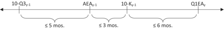
Our analyses rely on the intersection of four data sources: COMPUSTAT, CRSP, I/B/E/S, and EDGAR. This narrows the sample period to the years 1993–2017, corresponding to the range of 10-K file size data on EDGAR at the time of this study. We further narrow the universe to 151,963 firm-years with fourth and succeeding first quarter earnings announcement dates, and with 10-K and preceding third quarter 10-Q filing dates. As shown in Table 1 Panel A, we mitigate data errors by constraining each year y − 1 10-K filing date to: follow the year y − 1 earnings announcement date by no more than 3 months; precede the 1st quarter year y earnings announcement date by no more than 6 months; and follow the 3rd quarter year y − 1 10-Q filing date by no more than 8 months.16 These constraints reduce the sample by 4.4% from 151,963 to 145,268 firm-year observations. As further described in Table 1 Panel A, requiring each firm-year to have the stock price, returns, and analyst forecast data needed to implement our tests, further reduces the sample to 107,571 firm-years. Finally, requiring each 10-K's file size creates a base sample of 84,728 10-Ks filed by 5955 unique firms.
| Panel A: Firm-year observations associated with 10-K filings | ||
|---|---|---|
|
||
| (1) | Firm-years from 1993 to 2017, with non-missing earnings announcement dates for the 4th and 1st fiscal quarters and filing dates for the third quarter 10-Q and the 10-K (from COMPUSTAT) | 151,963 |
| (2) |
To alleviate data errors, observations must meet the following requirements:
These requirements restrict the number of firm-years to |
145,268 |
| (3) | Requiring firms to have stock returns data in CRSP and analyst following in I/B/E/S, further reduces the number of firm-years to | 107,571 |
| (4) | Requiring the 10-K file size to be available reduces the sample to 5955 unique firms and 84,728 firm-years |
84,728 Firm year |
| Panel B: Sample of analyst forecast revisions straddling 10-K filings | ||
|---|---|---|
|
||
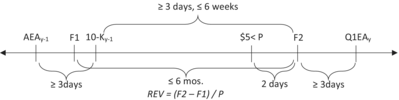
| (5) | We define a forecast revision as REV = (F2 − F1)/P, where F1 (F2) and P represent the older (newer) annual EPS forecast and stock price 2 days prior to the revision, respectively. We use I/B/E/S forecasts and require the firm to have stock price data on CRSP and both filing and announcement dates on COMPUSTAT. In addition to the restrictions in Panel A, we require each 10-K filing date to be straddled by at least one analyst's year y earnings forecast revision from the analyst's most recent forecast, F1, prior to the 10-K filing date to the analyst's first forecast, F2, following the 10-K filing date. From the initial 84,728 10-K filings described in Panel A, 37,323 filings are straddled by one or more (four, on average) individual analyst forecast revisions, subject to the constraint that F1 precedes F2 by no more than 6 months. This yields a sample of 148,044 analyst-firm-year observations | 148,044 |
| (6) | To create a relatively clean window defined by F1 and F2, we impose the following restrictions:
|
30,005 6072 15,492 |
| To alleviate the influence of penny stocks and potential data entry errors, we require the stock price 2 days prior to F2 to be at least $5, the revision, (F2 − F1)/P, to be less than 50%, and the forecast error, (A − F2)/P, to be less than 100% | 3977 | |
| The additional constraints, in step (6) reduce the 37,323 10-K filings derived in step 5 to 24,185 filings by 5225 unique firms. A total of 8342 unique analysts issue 92,498 forecast revisions that straddle these filings (3.8 revisions per filing, on average) | 92,498 | |
| Panel C: Selection criteria for subsamples used to evaluate H1 and H2 | No. obs. | |
|---|---|---|
|
||
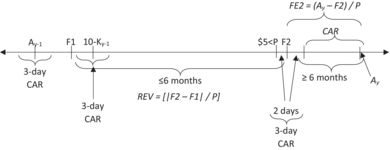
| (7) | We require data to calculate cumulated abnormal returns around the year y − 1 10-K filing date, the year y − 1 earnings announcement, and the forecast revision date. In addition, to calculate post-revision drift in abnormal returns, we require the future CAR, calculated from the second day after F2 (day +2) to the day after the firm announces the actual earnings that the analyst is forecasting (Ay), to have an accumulation period of at least 6 months. These requirements reduce the 92,498 analyst-firm-year observations from step (6) by 961 observations | 961 |
| Subtotal | 91,537 | |
| (8) | To alleviate the influence of outliers, we also omit observations in which the absolute studentised residual from OLS estimation of the basic model exceeds 3 (this omits 1.7% of the 91,537 observations from step (7) above | 1576 |
| The final number of analyst-firm-year observations used to evaluate H1 and H2 is | 89,961 | |
Next, we select analyst forecast revisions associated with each of the 84,728 10-K filings identified above. As described in Table 1 Panel B, we define a forecast revision as (F2 − F1)/P, where F2 (F1) is an individual analyst's new (prior) forecast of year y earnings, and P is the stock price 2 days prior to the date F2 is issued.17 We focus on forecast revisions that straddle each 10-K filing, meaning F1 (F2) precedes (follows) the filing date.
To alleviate confounding effects from information at earnings announcement and 10-K filing dates, Table 1 Panel B shows that we impose the following constraints: F2 precedes the upcoming 1st quarter earnings announcement; F1 and F2 are separated by no more than 6 months; F2 is at least 3 days and no more than 6 weeks later than the 10-K filing date, and at least 3 days earlier than the 1st quarter earnings announcement; and the 10-K filing date follows the annual earnings announcement by at least 3 days. We also eliminate observations where the price deflator is less than $5. Consistent with prior research, we alleviate the influence of data entry errors, by omitting observations in which either the revision ((F2 − F1)/P) exceeds 50% or the price-scaled forecast error ((A − F2)/P) exceeds 100%. This selection procedure yields a sample of 92,498 analyst-firm-year forecast revision observations straddling 24,185 10-K filings and issued by 8342 unique analysts following 5225 firms (on average, 3.8 forecast revisions per 10-K filing).
As described in Table 1 Panel C, we require data to estimate cumulative abnormal returns (CAR) over the 3 days centred on the 10-K filing, annual earnings announcement, and forecast revision dates. In addition, to calculate post-revision drift, we require data to estimate CAR from the second day following F2 to the day after the firm announces the actual earnings (Ay) that the analyst is forecasting. We also omit observations in which the absolute studentised residual from ordinary least squares (OLS) estimation of our basic market efficiency models exceeds three. Applying these constraints causes an approximate 2% decline from 92,498 observations in the forecast revisions sample to the final sample of 89,961 observations with sufficient returns and forecast revisions data to evaluate H1 and H2.
5 RESEARCH DESIGN
5.1 Measuring complexity
As described by Loughran and McDonald (2024, p. 2), “complexity is a broad and amorphous concept that is difficult to quantify”. The overall complexity of 10-K information increases with the firm's underlying operating complexity (Hoitash & Hoitash, 2022; Huang et al., 2018), efforts to comply with complex accounting policy promulgated by accounting regulators (Chychyla et al., 2019), and the complexity of discretionary disclosures associated with the application of accounting policies (Cazier & Pfeiffer, 2016). Prior studies measure overall 10-K complexity with reference to the Gunning Fog Index (Bushee et al., 2018; Gao et al., 2023; Lehavy et al., 2011; Li, 2008); the Bog Index (Bonsall et al., 2017); XBRL diversity (Hoitash & Hoitash, 2018); the intensity of complexity-related word usage with reference to a researcher-specified list of complexity-related words (Loughran & McDonald, 2024); word count (You & Zhang, 2009); gross file size (Loughran & McDonald, 2014); gross file size, net of space allocated to tables, charts, and figures (Bae et al., 2023; Loughran & McDonald, 2016); and scarcity of quantification within the 10-K's textual disclosures (Siano & Wysocki, 2018).
As described by Loughran and McDonald (2024), the Fog Index suffers from identifying as complex words, simple to understand frequently used multisyllable words like “including and agreement,” and both the Fog and Bog Indexes suffer from identification of generally accepted readability-enhancing financial jargon as complexity-increasing (Loughran & McDonald, 2014).18 Net file size suffers from broad-based elimination of charts, figures, and tables which can constitute a large component of complex information in many 10-Ks. Prior studies find high correlations between gross and net file size (Loughran & McDonald, 2014) and between net file size and word count (Loughran & McDonald, 2024). Given the high correlations among complexity measures and a desire to avoid subjectivity and other pitfalls associated with net file size, Fog Indexes, and Bog Indexes, we use gross file size to proxy for financial reporting complexity.19 Across three levels of gross 10-K file size, we examine the degree to which analyst and market efficiency with respect to 10-K information depends on financial reporting complexity.20
5.2 Evaluating H1
As shown in Table 1 Panel C, the variable represents the price-deflated signed error in analyst a's first year y earnings forecast, , following f's year y − 1 10-K filing date. represents the target of , and represents f's closing stock price as of the second day prior to the date I/B/E/S associates with . The variable represents the analyst's forecast revision, where represents a's most recent forecast of f's year y earnings preceding the 10-K filing date, meaning the revision straddles the 10-K filing date. In Equation (1), our coefficient of interest is , which captures the extent of analyst underreaction to the information underlying the forecast revision.
Following Abarbanell and Bernard (1992), we transform into percentiles on a scale of zero (smallest percentile) to one (largest percentile) before estimating models containing .21 We also transform into percentiles placed on a scale of zero to one. As shown in(1), has three earnings news components: predictable optimism/pessimism bias, captured by the intercept, ; predictable underreaction, captured by analyst a's underreaction coefficient, , times the 10-K information variable, ; and an unpredictable earnings shock represented by the residual, .
In regression models (1) and (2) above, the Controls vector includes year fixed effects to mitigate potential omitted variable bias caused by excluding unobserved variables that evolve over time but are constant across firms (e.g., macroeconomic or regulatory trends). It also includes analyst-firm fixed effects to mitigate unobservable time-invariant heterogeneity across analyst-firm pairs. To mitigate identification issues and control for the contemporaneous returns-revision relation, the Controls vector includes a variable indicating the quintile of the 3-day abnormal return () centered on the date of and interacted with S, M, and L, our 10-K file size indicator variables.
To control for the You and Zhang (2009) good/bad news signal (discussed below), the Controls vector includes , a variable indicating the quintile of the 3-day abnormal return around the filing date, interacted with S, M, and L, our 10-K file size indicator variables. To control for post-earnings announcement drift and analyst underreaction to news around the time of the annual earnings announcement (e.g., Abarbanell & Bernard, 1992), the Controls vector includes , a variable indicating the quintile of the 3-day abnormal return around the most recent earnings announcement. The time between pre- and post-filing forecasts varies across analysts. We control for this variation by including the number of days from F1 to the 10-K filing date () and the number of days from the 10-K filing date to F2 (). In addition, we control for the number of days from the annual earnings announcement to the 10-K filing (Days_AEA_10-Kfy) and the number of days from the 10-K filing to the upcoming first quarter earnings announcement ().22
5.3 Evaluating H2
H2 examines market efficiency with respect to 10-K information and whether the impact of analyst underreaction on market efficiency increases with 10-K complexity. We measure analyst impact as the difference between market underreaction coefficients in regressions with and without controls for analyst underreaction. Our tests evaluate whether this difference increases with 10-K complexity.
As described in (1), contains a predictable component that is correlated with the information underlying the analyst's forecast revision () and a shock () that is uncorrelated to this information. Since captures the market's response to the predictable component of , estimates the ERC and should have approximately the same value as in (6).23
As described by Shane and Brous (2001), including in (7) controls for the relation between and . Thus, in (6) controls for analyst underreaction to the 10-K information reflected by . then simulates the market underreaction coefficient, without the influence of analyst underreaction, and in (6) minus in (7) estimates the impact of analyst underreaction on market efficiency with respect to 10-K information reflected by . Using a difference-in-differences research design and bootstrapping techniques described in MacKinnon et al. (2018) and Ng and Wilcox (2012), we estimate whether the difference between and significantly increases with 10-K complexity.
6 RESULTS
Table 2 Panels A and B, respectively, present descriptive statistics and a correlation matrix describing the variables used to evaluate H1 and H2. Panel A shows cumulative abnormal returns (CAR) over the period from 2 days following an analyst's 10-K-straddling earnings forecast revision (Rev) through the day following the next year's earnings announcement averaging about 1%, Rev averaging around −0.4%, and the analyst's earnings forecast error, FE2, (calculated over the same period as CAR) averages around −0.5%. The means of Rev and FE2 indicate a slight analyst optimism bias, although the median of both statistics is zero (i.e., unbiased).
| Panel A: Descriptive statistics for variables identified with tests of H1 and H2 (sample size = 89,961 observations) | |||||||
|---|---|---|---|---|---|---|---|
| Variable | Mean | SD | p10 | p25 | p50 | p75 | p90 |
| CAR | 0.009 | 0.315 | −0.335 | −0.140 | 0.014 | 0.165 | 0.346 |
| FE2 | −0.005 | 0.035 | −0.033 | −0.009 | 0.000 | 0.005 | 0.018 |
| Rev | −0.004 | 0.030 | −0.014 | −0.004 | 0.000 | 0.001 | 0.005 |
| Fsize | 2,300,692 | 2,417,355 | 199,575 | 681,525 | 1,709,067 | 3,066,510 | 4,939,240 |
| RevCAR | −0.003 | 0.058 | −0.049 | −0.020 | −0.001 | 0.018 | 0.045 |
| 10-K_CAR | 0.000 | 0.039 | −0.035 | −0.016 | 0.000 | 0.016 | 0.036 |
| AEA_CAR | 0.003 | 0.071 | −0.072 | −0.030 | 0.002 | 0.036 | 0.076 |
| Days_10-K_F2 | 28.148 | 16.056 | 8 | 14 | 27 | 41 | 51 |
| Days_F1_10-K | 38.336 | 35.384 | 7 | 15 | 27 | 46 | 100 |
| Days_AEA_10-K | 27.542 | 14.928 | 8 | 16 | 26 | 36 | 49 |
| Days_10-K_Q1EA | 54.576 | 14.025 | 34 | 47 | 56 | 64 | 70 |
| Days_F2_Q1EA | 26.428 | 15.525 | 8 | 14 | 23 | 37 | 49 |
| Panel B: Correlations among key variables | |||||||||||
|---|---|---|---|---|---|---|---|---|---|---|---|
| Variable | CAR | FE2 | Rev | Fsize | RevCAR | 10-K_CAR | AEA_CAR | 10-K_F2 | F1_10-K | AEA_10-K | 10-K_Q1EA |
| CAR | 1.000 | ||||||||||
| FE2 | 0.275 | 1.000 | |||||||||
| Rev | 0.008 | 0.130 | 1.000 | ||||||||
| Fsize | −0.008 | 0.010 | 0.014 | 1.000 | |||||||
| RevCAR | 0.019 | 0.091 | 0.116 | 0.021 | 1.000 | ||||||
| 10-K_CAR | 0.011 | 0.067 | 0.115 | 0.032 | 0.034 | 1.000 | |||||
| AEA_CAR | 0.002 | 0.058 | 0.073 | −0.029 | 0.019 | 0.032 | 1.000 | ||||
| Days_10-K_F2 | 0.002 | 0.031 | 0.016 | 0.186 | 0.006 | 0.020 | 0.004 | 1.000 | |||
| Days_F1_10-K | 0.007 | −0.007 | −0.032 | −0.110 | −0.016 | −0.021 | 0.016 | −0.214 | 1.000 | ||
| Days_AEA_10-K | 0.027 | −0.013 | −0.026 | −0.163 | −0.044 | −0.031 | −0.021 | −0.309 | 0.249 | 1.000 | |
| Days_10-K_Q1EA | −0.017 | 0.000 | 0.040 | 0.401 | 0.020 | 0.039 | 0.000 | 0.373 | −0.214 | −0.557 | 1.000 |
| Days_F2_Q1EA | −0.022 | −0.016 | 0.015 | 0.183 | 0.019 | 0.008 | −0.003 | −0.545 | −0.025 | −0.309 | 0.501 |
The interquartile range and standard deviation indicate substantial variation in 10-K file size across the firm-years in our sample. On average, analysts take 28 days to revise their forecasts following a 10-K filing, and the age of the forecast preceding the 10-K filing is about 38 days. The periods between annual earnings announcements and subsequent 10-K-filings and between 10-K filings and upcoming first quarter earnings announcements average 28 and 55 days, respectively. Finally, the horizon between a revised forecast and the upcoming first quarter earnings announcement averages 26 days.
The correlation matrix in Table 2 Panel B shows a strong contemporaneous relation between the analyst's earnings forecast error, FE2, and the contemporaneous cumulative abnormal return, CAR, suggesting that the analyst's unexpected earnings is a reasonable proxy for the market's earnings surprise. The positive univariate correlations between Rev and both FE2 and CAR suggest significant underreaction by both the market and analysts. Multivariate tests of H1 and H2 formally evaluate this conjecture. Tests of H1 evaluate whether analyst underreaction increases with 10-K complexity, and tests of H2 examine whether analyst underreaction significantly impacts market efficiency and whether this impact grows with 10-K complexity.
Most of the control variables are significantly correlated with Rev, FE2, and CAR and the directions of univariate correlations among control variables are unsurprising. One of these control variables is the lag in days between the 10-K filing date and the analyst's first revised forecast following the 10-K filing date (Days_10-K_F2). As shown in Table 2 Panel B, the univariate correlation between Days_10-K_F2 and the 10-K file size is 18.6%, which strongly indicates that analysts take significantly more time to revise forecasts following more complex 10-K filings. Another control variable is the You and Zhang (2009) proxy for the information content of the 10-K; that is, the 10-K-straddling three-day stock return which we label 10-K_CAR. Rev and 10-K_CAR have a statistically significant 11% univariate correlation, leaving substantial room for these two proxies to reflect different aspects of the information in the 10-K. Since our proxy allows time for analysts to digest the 10-K's information, we argue that it is more likely to reflect the earnings implications of the complex information in the 10-K and is, therefore, more appropriate for our purposes.
6.1 Does analyst underreaction increase with 10-K complexity (H1)?
Table 3 column (1) shows the results of estimating Model (2) to evaluate H1. Consistent with H1, estimates of Model (2) coefficients show that analysts underreact to the information underlying their own 10-K-straddling forecast revisions and the underreaction increases with 10-K complexity. The analyst's underreaction coefficient on the information variable, , increases monotonically from 0.0126 for earnings forecast revisions straddling 10-K filings in the lowest tercile of the file size distribution to 0.0155 for the middle file size tercile and 0.0191 for the largest file size tercile. Thus, the analyst underreaction coefficient on revisions straddling high-complexity 10-Ks is (an economically and statistically significant) 52% higher than the coefficient on revisions straddling low-complexity 10-Ks. This result is consistent with the inference that, due to greater uncertainty regarding the earnings implications of complex 10-K information, analysts' forecast revisions underreact to a greater extent with reference to high-complexity 10-Ks than they do with reference to low-complexity 10-Ks. The earnings uncertainty effect of complexity on analyst underreaction apparently outweighs any reduction in underreaction due to more able analysts following more complex firms.
| Model (2) | Model (8) | Model (9) | ||||
|---|---|---|---|---|---|---|
| Test of H1 | Test of H2 | Test of H2 | ||||
| FE2 | CAR | CAR | ||||
| Intercept | −0.0074*** | −2.806 | 0.0427** | 2.184 | 0.1250*** | 6.439 |
| S | 0.0032*** | 3.371 | 0.0090 | 1.088 | 0.0068 | 0.828 |
| L | −0.0019* | −1.938 | 0.0121 | 1.548 | 0.0186** | 2.433 |
| Rev*S | 0.0126*** | 11.788 | 0.0060 | 0.596 | −0.0495*** | −4.884 |
| Rev*M | 0.0155*** | 13.345 | 0.0408*** | 4.428 | −0.0157* | −1.688 |
| Rev*L | 0.0191*** | 16.666 | 0.0391*** | 4.443 | −0.0305*** | −3.494 |
| *S | 3.4002*** | 22.817 | ||||
| *M | 3.0180*** | 24.347 | ||||
| *L | 2.9016*** | 24.681 | ||||
| FE2*S | 3.3103*** | 22.310 | ||||
| FE2*M | 2.9817*** | 24.211 | ||||
| FE2*L | 2.8110*** | 24.238 | ||||
| RevCAR*S | 0.0019*** | 3.002 | −0.0082 | −1.136 | −0.0149** | −2.059 |
| RevCAR*M | 0.0045*** | 5.896 | 0.0093 | 1.251 | −0.0026 | −0.354 |
| RevCAR*L | 0.0040*** | 4.841 | 0.0114 | 1.593 | 0.0040 | 0.553 |
| 10-K_CAR*S | 0.0020*** | 3.321 | −0.0026 | −0.351 | −0.0061 | −0.845 |
| 10-K_CAR*M | −0.0004 | −0.596 | −0.0078 | −1.096 | −0.0145** | −2.045 |
| 10-K_CAR*L | 0.0026*** | 3.171 | 0.0141* | 1.958 | 0.0075 | 1.044 |
| AEA_CAR | 0.0014*** | 3.259 | −0.0287*** | −6.897 | −0.0359*** | −8.631 |
| Days_10-K_F2 | 0.0138** | 2.295 | −0.1126*** | −3.864 | −0.1930*** | −6.650 |
| Days_F1_10-K | 0.0006 | 0.810 | 0.0009 | 0.112 | −0.0023 | −0.296 |
| Days_AEA_10-K | −0.0033 | −1.379 | 0.0082 | 0.422 | −0.0169 | −0.873 |
| Days_10-K_Q1EA | −0.0177*** | −2.605 | 0.0481* | 1.821 | 0.1000*** | 3.788 |
| Days_F2_Q1EA | 0.0134* | 1.901 | −0.1407*** | −4.182 | −0.2260*** | −6.738 |
| Analyst-firm pair fixed effects | Included | Included | Included | |||
| Year fixed effects | Included | Included | Included | |||
| N | 89,961 | 89,961 | 89,961 | |||
| Analyst-firm clusters | 50,036 | 50,036 | 50,036 | |||
| Adjusted R-squared | 0.0685 | 0.0905 | 0.0892 | |||
-
Note: Standard errors clustered at the analyst-firm pair level. Tests of H1 and H2 rely on estimates from Models (2), (8), and (9) described in the text and reproduced below. All variables are defined in the Appendix, and Table 1 Panel C depicts the dependent variable and test variables on a timeline.
- *p-value < 0.10, **p-value < 0.05, ***p-value < 0.01.
6.2 Does analyst impact on market efficiency increase with 10-K complexity (H2)?
Table 3 columns (2) and (3) report the results of estimating Models (8) and (9) to evaluate H2. As described in subsection 5.3 above, Models (8) and (9) differ only because (8) includes the earnings shock, , from Model (2); whereas, (9) includes the entire analyst forecast error, . Both Models (8) and (9) regress future returns on , but the coefficient on takes on different meanings depending on whether or is in the model.
As described in subsection 5.2, since and are uncorrelated, , the coefficient on in Model (8), measures the ERC times the market's underreaction coefficient, including the impact of analyst underreaction; that is, the relation between and is not controlled. Since the coefficient on measures the ERC, effectively estimates the market underreaction coefficient, including the impact of analyst underreaction. Including in Model (9) controls for the relation between and , so the coefficient, , on in Model (9) measures the ERC times the market's underreaction coefficient, excluding the impact of analyst underreaction, and the coefficient, , on estimates the ERC. Thus, in (9) approximates in (8); in (8) provides an estimate of the market underreaction coefficient, excluding the impact of analyst underreaction; and provides an estimate of the impact of analyst underreaction on market efficiency with respect to the information reflected by .
Models (8) and (9) allow estimation of analyst impact within 10-K file size terciles, so estimates the difference in the impact of analyst underreaction on market efficiency with respect to 10-K information underlying for observations associated with large 10-K file sizes (proxying for high-complexity 10-K information) versus observations associated with small 10-K file sizes (proxying for low-complexity 10-K information). In our tests of H2, finding that is greater than zero is consistent with the impact of analyst underreaction on market efficiency increasing with 10-K complexity. Table 4 summarises the results of estimating Models (8) and (9) in Table 3.
| Smallest 10-K size tercile (i.e., low complexity) | Largest 10-K size tercile (i.e., high complexity) | |
|---|---|---|
| in model (8), where = the market underreaction coefficient, including the impact of analyst underreaction | 0.0060 | 0.0391*** |
| in Model (8) | 3.400*** | 2.902*** |
| 0.0018 | 0.0135*** | |
| in model (9), where = the market underreaction coefficient, excluding the impact of analyst underreaction | −0.0495*** | −0.0305*** |
| in Model (9) | 3.3103*** | 2.8110*** |
| −0.0150*** | −0.0108*** | |
| = analyst impact on market efficiency | 0.0167*** | 0.0243*** |
- *p-value < 0.10, **p-value < 0.05, ***p-value < 0.01.
While Table 4 shows that analyst underreaction significantly impacts the market response to information underlying analyst forecast revisions straddling both low- and high-complexity 10-K filings, the impact associated with large file size (high-complexity) 10-Ks is 45% higher than the impact associated with small file size (low-complexity) 10-Ks and the difference is statistically significant with a p-value less than 0.01 (estimated with bootstrapping techniques in Table 5).
| Estimation of market inefficiency with and without the impact of analysts' underreaction | ||||||
|---|---|---|---|---|---|---|
| Dependent variable: CAR | Observed coefficient | Clustered std. err. | Z-statistic | p-Value > |Z| | 95% confidence interval | |
| 0.0018 | 0.0026 | 0.67 | 0.503 | −0.0034 | 0.0069 | |
| 0.0135 | 0.0028 | 4.88 | 0.000 | 0.0081 | 0.0189 | |
| −0.0150 | 0.0027 | −5.52 | 0.000 | −0.0203 | −0.0096 | |
| −0.0108 | 0.0029 | −3.8 | 0.000 | −0.0164 | −0.0052 | |
| Bootstrap uses 89,961 observations with 10,000 replications based on 50,036 analyst-firm clusters | ||||||
|---|---|---|---|---|---|---|
| Dependent variable: CAR | Observed coef. | Bootstrap std. err. | Z-statistic | p-Value > |Z| | Normal-based (95% confidence interval) | |
| 0.0018 | 0.0030 | 0.59 | 0.553 | −0.0041 | 0.0076 | |
| 0.0135 | 0.0030 | 4.54 | 0.000 | 0.0077 | 0.0193 | |
| −0.0150 | 0.0031 | −4.88 | 0.000 | −0.0210 | −0.0090 | |
| −0.0108 | 0.0031 | −3.53 | 0.000 | −0.0169 | −0.0048 | |
| 0.0243 | 0.0002 | 129.03 | 0.000 | 0.0239 | 0.0247 | |
| 0.0167 | 0.0002 | 88.48 | 0.000 | 0.0164 | 0.0171 | |
| Impact difference | 0.0076 | 0.0003 | 28.36 | 0.000 | 0.0071 | 0.0081 |
An interesting implication that emerges from our evidence in Table 4 is that the impact of analyst underreaction on market efficiency with respect to 10-K information increases with 10-K complexity. We find that, controlling for the impact of analyst underreaction, the market overreacts to information underlying forecast revisions straddling both low- and high-complexity 10-Ks with statistically significant overreaction coefficients of −0.0150 and − 0.0108, respectively. Without controlling the impact of analyst underreaction: (i) the simulated market overreaction to low-complexity 10-K information disappears with an insignificant underreaction coefficient estimated at 0.0018; and (ii) the simulated market overreaction to high-complexity 10-K information has significant underreaction with an underreaction coefficient estimated at 0.0135. This evidence is consistent with analyst underreaction mitigating market overreaction to low-complexity 10-K information and fully explaining market underreaction to high-complexity 10-K information.
Overall, our tests of H1 and H2 produce evidence consistent with the following mechanism giving rise to market underreaction to the earnings implications of high-complexity 10-K filings. First, the underreaction-increasing uncertainty associated with the earnings implications of high-complexity 10-K information outweighs the underreaction-decreasing greater ability of analysts attracted to following firms with complex 10-Ks, leading to a positive relation between 10-K complexity and analyst underreaction. Second, investors rely more heavily on analysts for the interpretation of more complex 10-K information, investors do not effectively unravel the underreaction in analysts' earnings forecasts, and we observe an impact of analyst underreaction on market efficiency that increases with 10-K complexity. Third, this greater impact on stock prices fully explains price discovery-compromising market underreaction to the earnings implications of information underlying analysts' 10-K-straddling earnings forecast revisions.
7 CONCLUSION
Over the last two decades, 10-K complexity has received the attention of regulators (FASB, 2012, 2018, 2024; SEC, 2008, 2018), journalists (e.g., Monga & Chasan, 2015), and academic researchers (e.g., Cazier & Pfeiffer, 2016; Hoitash et al., 2021; Lehavy et al., 2011; Loughran & McDonald, 2014; You & Zhang, 2009). This paper provides justification for concern over increasing 10-K complexity by drawing attention to a cost in the form of increased analyst underreaction to the 10-K's earnings implications and compromised price discovery in capital markets. Our research question is important, because financial analysts can either mitigate or foster market inefficiency with respect to increasingly complex 10-K information. Our evidence suggests that analyst forecasting behaviour mitigates market overreaction to less complex 10-K information and fosters market underreaction to more complex 10-K information.
The analyst's 10-K-straddling earnings forecast revision serves as our proxy for the earnings implications of the information in the 10-K. The analyst's underreaction coefficient measures the relationship between the 10-K-straddling earnings forecast revision and the subsequent forecast error defined by the next year's actual earnings minus the analyst's first earnings forecast following the 10-K filing date. In tests of our first hypothesis, we find that this underreaction coefficient is an economically and statistically significant 52% higher among observations associated with more complex (top tercile) 10-K filings, as compared to the underreaction coefficient among observations associated with less complex (bottom tercile) 10-K filings; that is, analyst underreaction increases with 10-K complexity. These results are consistent with prior research findings that uncertainty in analysts' earnings forecasts breeds underreaction (Raedy et al., 2006; Zhang, 2006), and 10-K complexity breeds uncertainty in analysts' earnings forecasts (Bae et al., 2023; Hoitash et al., 2021; Lehavy et al., 2011). Our results suggest that the underreaction-increasing effect of increased uncertainty associated with the earnings implications of more complex 10-K filings outweighs the underreaction-decreasing effects of greater analyst following and greater analyst effort documented in Lehavy et al. (2011).
Our research design highlights a technique that estimates the market's underreaction coefficient with and without controls for analyst underreaction. Using this technique, we find that without the influence of analyst underreaction, stock prices immediately after the analyst's revised forecast following the 10-K filing exhibit significant overreaction to the earnings implications of the 10-K information. Removing the model's control for analyst underreaction allows detection of the influence of analyst underreaction on market prices. Allowing this influence, our evidence indicates that analyst underreaction mitigates what would have been market overreaction to the earnings implications of less complex 10-K information, and analyst underreaction overwhelms what would have been market overreaction to more complex 10-K information, leading to significant market underreaction. The significant market underreaction to more complex 10-K information compromises price discovery and can, thereby, lead to a misallocation of investor resources.
Our study is not without limitations. First, we infer the efficiency of analysts' earnings forecasts and stock prices with respect to the earnings implications of the information contained in high- versus low-complexity 10-K filings, without directly observing the behaviour of analysts and investors. Therefore, our proxies for under/overreaction and for the earnings implications of 10-K information necessarily contain measurement error, which compromises their construct validity. However, we have no reason to believe this measurement error biases our tests towards rejection of our hypotheses. Second, as in all archival empirical studies, in spite of our best efforts to include control variables, unknown correlated omitted variables undoubtedly exist. Again, we have no reason to believe that these omitted variables bias our results towards rejection of our hypotheses. Third, the analysts selecting to follow firms with complex 10-Ks may be better analysts who tend to underreact less. If that is the case, then failure to control for this selection bias works against the power of our tests for greater uncertainty-driven analyst underreaction to more complex 10-K information. We do not control for analyst ability, because we want to allow analyst ability to alleviate underreaction to more complex 10-K filings. This creates tension in our tests examining whether analyst underreaction increases with 10-K complexity.
Finally, this study, as well as Raedy et al. (2006) and Bernhardt et al. (2016), assumes analysts have asymmetric reputation costs of forecast inaccuracy, whereby investors penalise them to a greater extent for inaccuracy stemming from overreaction versus underreaction to information with implications for a firm's future earnings. Future research might revisit the evidence in Hong et al. (2000) and Mikhail et al. (2003) suggesting that more accurate analysts experience better career outcomes. Future research can assess whether the positive relation between forecast inaccuracy and job turnover becomes more pronounced for observations where overreaction versus underreaction led to the inaccuracy.
Overall, we believe that we have compelling evidence supporting the following mechanism underlying market underreaction to high-complexity 10-K filings: increased information uncertainty outweighs greater analyst ability and analyst underreaction to 10-K information increases with 10-K complexity, investors rely more heavily on analyst interpretation of more complex 10-K information and do not adjust out analyst underreaction when responding to analysts' earnings forecast revisions, the market would overreact to 10-K information without the influence of analysts, analyst underreaction offsets what would have been market overreaction to the earnings implications of low-complexity 10-K information, and analyst underreaction overwhelms what would have been market overreaction to high-complexity 10-K information, leading to significant underreaction that compromises price discovery in capital markets.
ACKNOWLEDGEMENTS
We are grateful for comments from Michael Clement, Ro Gutierrez, Charles Lee, Edward Li, K. Ramesh, Anne Wyatt, and workshop participants at Monash University, Queensland University, UC-Berkeley, and Virginia Commonwealth University, as well as financial support from the Frank Wood Accounting Research Fund at the Raymond A. Mason School of Business, William and Mary. We also thank Jeremy Bettis at Google for code to access 10-K file-sizes.
APPENDIX: VARIABLE DEFINITIONS
| Evaluate variables | |
| represents the within-sector percentile rank (on a zero–one scale) of analyst a's year y earnings forecast revision that straddles firm f's year y − 1 10-K filing date. F1 (F2) is analyst a's closest year y earnings forecast preceding (following) firm f's year y − 1 10-K filing date. The revision is scaled by the firm's closing stock price, 2 days prior to the revision date | |
| Fsize f,y−1 | 10-K file size, in bytes, for fiscal year y − 1 |
| S, M, L | S = 1, if Fsizef,y−1 is in the lowest tercile of its within-sector distribution, and S = 0 otherwise; M = 1, if Fsizef,y−1 is in the middle tercile of its within-sector distribution, and M = 0 otherwise; and L = 1, if Fsizef,y−1 is in the highest tercile of its within-sector distribution, and L = 0 otherwise |
| The residual from estimating the regression of FE2 on Rev and Control variables; that is, the regression Model (1) used to evaluate H1 | |
| Dependent variables | |
| Firm f's characteristics-adjusted return from day t + 2 after analyst a's forecast revision through the day after the firm announces the actual EPS that the analyst is forecasting | |
| The signed error in the revised one-year-ahead forecast (F2) issued by analyst a relative to firm f's actual annual EPS (per I/B/E/S) scaled by the firm's closing stock price 2 days prior to the forecast revision date | |
| Control variables | |
| A categorical variable that ranks firm f's cumulative abnormal return (CAR) during the 3 days around the forecast revision date relative to the CARs of other firms in the same fiscal year. We assign values of −0.5, −0.25, 0, 0.25 and 0.5 to the 1st, 2nd, 3rd, 4th, and 5th quintiles, respectively | |
| A categorical variable that ranks firm f's cumulative abnormal return during the 3 days around the10-K filing date relative to that of other firms in the same fiscal year. The lowest, 2nd, 3rd, 4th, or highest quintile equal −0.5, −0.25, 0, 0.25 or 0.5, respectively | |
| A categorical variable that ranks firm f's cumulative abnormal return during the 3 days around the annual earnings announcement date relative to that of other firms in the same fiscal year. The lowest, 2nd, 3rd, 4th, or highest quintile equal −0.5, −0.25, 0, 0.25 or 0.5, respectively | |
| Number of days between firm f's year y − 1 10-K filing date and the upcoming first-quarter interim earnings announcement for year y, scaled by the range of days for all firms filing year y − 1 10-Ks | |
| Number of days between firm f's annual earnings announcement and its year y − 1 10-K filing, scaled by the range of days for all firms filing year y − 1 10-Ks | |
| Number of days between the10-K filing date and analyst a's forecast revision date, scaled by the range of days for all revisions following year y − 1 10-Ks filed | |
| Number of days from analyst a's newest pre-10-K filing forecast (i.e., F1) to the 10-K filing date, scaled by the range of days for all F1 revisions preceding year y − 1 10-Ks | |
| Number of days from the forecast revision date to the upcoming first-quarter interim earnings announcement, scaled by the range of days for all revisions following year y − 1 10-Ks | |
Open Research
DATA AVAILABILITY STATEMENT
All data underlying this studies results and inferences are available from public sources.
REFERENCES
- 1 Similar to You and Zhang (2009) but with reference to 10-Q rather than 10-K filings, Lee (2012) produces evidence of complexity-related market underreaction to the information reflected by the 10-Q-straddling 3-day stock return. Like You and Zhang (2009), Lee (2012) does not examine the efficiency of analyst forecasts or the impact of complexity-related analyst underreaction on market efficiency with respect to the earnings implications of the filing.
- 2 Contrary to Miller (2010), You and Zhang (2009) find that abnormal trading volume increases with 10-K complexity. You and Zhang (2009) do not separately analyse small and large investor trades.
- 3 Huddart et al. (2007), You and Zhang (2009), and Cazier and, Pfeiffer (2016) use the three-day stock return centred on the 10-K filing date to proxy for value-relevant information released with the 10-K, Livnat and Mendenhall (2006) use analysts' forecast errors to proxy for value-relevant information released at the time of an earnings announcement. Keskek and Tse (2024) and Chen et al. (2020) use analysts' forecast revisions to proxy for value-relevant information underlying those revisions.
- 4 In particular, Lehavy et al. (2011) find that as readability declines, the proportion of a firm's stock returns related to analyst forecast revisions to the total firm's stock return during the time period between the 10-K filing and the subsequent fiscal year-end increases.
- 5 Two prior studies, reaching opposite conclusions, examine the information content of analysts' research output following 10-K filings. Lehavy et al. (2011) find that the information content of analysts' revised forecasts following 10-K filings increases with 10-K complexity; whereas, Hoitash et al. (2021) find that the information content of analysts' revised stock recommendations following 10-K filings declines with 10-K complexity. Thus, whether investor reliance on analysts increases with 10-K complexity is an open question.
- 6 Bradshaw et al. (2017, p. 158) calls for archival research that integrates empirical implications from models of analyst underreaction such as the one developed in Raedy et al. (2006).
- 7 Like Trueman (1990), Abarbanell (1991) explains analyst underreaction in terms of overweighting the analyst's private information. Abarbanell's (1991) theory assumes investors prefer analysts' forecasts that reveal the analysts' private information and ignore conflicting signals from public information. In contrast to Trueman (1990) and Abarbanell (1991), Aharoni et al. (2017) analytically demonstrate plausible conditions leading top analysts to underweight their private information so as to avoid free riding by less-informed rival analysts.
- 8 Also see Chen and Jiang (2006), who argue that purposeful misweighting of the analyst's private versus public information increases with the forecast horizon, because investors punish inaccuracy more severely as the horizon shortens.
- 9 Cazier and Pfeiffer (2016, p. 4) confirm You and Zhang (2009), but only when 10-K complexity is measured with reference to residual disclosure stemming “primarily from discretionary managerial choices”.
- 10 The time between the 10-K filing date and the analyst's first post-10-K filing forecast averages 28 days in our sample as a whole, with significantly longer delays in analyst response to high-complexity 10-K filings.
- 11 In untabulated analysis (available upon request), we find a strong relation between 10-K complexity and return volatility during the year ending with the 10-K balance sheet date (p-value < 0.01). Thus, 10-K complexity is associated with increased uncertainty around the analyst's earnings expectations.
- 12 Raedy et al. (2006) model underreaction as a rational analyst response to investor-driven incentives; whereas, Zhang (2006) treats underreaction as a phenomenon that arises from analysts' irrational behavioural biases. Both papers find that underreaction increases with uncertainty in earnings expectations. Zhang (2006) relies on dispersion in analysts' forecasts to proxy for uncertainty, whereas Raedy et al. (2006) use the forecast horizon to proxy for uncertainty.
- 13 Similarly, Barth et al. (2001) find that firms with more difficult-to-forecast earnings and greater uncertainty around earnings forecasts attract greater analyst following and greater analyst effort; that is, analysts are attracted to following firms where they have more to contribute.
- 14 In an analysis of the market reaction to analysts' buy-sell-hold stock recommendations, Hoitash et al. (2021) reach the opposite conclusion; that is, the market responds less intensely to analysts' stock recommendation revisions following more complex 10-K filings. The contradiction of the Lehavy et al. (2011) information content result might be due to the more recent time period underlying the Hoitash et al. (2021) sample (Loughran & McDonald, 2014).
- 15 Lee (2012) studies the stock market reaction to 10-Q filings and provides evidence of price drifts in the direction of the 10-Q-straddling 3-day stock return that increase with measures of 10-Q complexity. Lee (2012) also finds that greater analyst following mitigates the complexity-related underreaction in stock prices. This reinforces our observation that the Lehavy et al. (2011) evidence of analyst following increasing with 10-K complexity works against the power of tests of our hypothesis predicting underreaction in analysts' earnings forecasts that increases with 10-K complexity.
- 16 Throughout the paper, the subscript, y, represents the year with the forecasted earnings, and the subscript, y − 1, represents the year associated with the 10-K balance sheet date.
- 17 Throughout the paper, days refer to trading days.
- 18 During an expanded sample period and using the Fog Index to measure complexity as in Lehavy et al. (2011), Loughran and McDonald (2014) fail to find evidence confirming the negative (positive) relation between complexity and forecast accuracy (dispersion) following 10-K filing dates documented by Lehavy et al. (2011). However, Loughran and McDonald (2014) do find confirming evidence of these relations using gross file size, thus supporting the efficacy of gross file size as an omnibus measure of complexity. Similarly, Miller (2010) includes the complexity proxies, Fog Index and gross file size, in a model predicting that abnormal trading volume around the time of the 10-K filing date declines with 10-K complexity. Miller (2010) finds evidence consistent with this prediction when the Fog Index proxy is in the model alone; however, after adding gross file size to the model, the Fog Index variable is no longer significantly related to abnormal trading volume and the gross file size proxy remains significant. Miller (2010, p. 2109) interprets this evidence as suggesting “the measures are substitutes, but the effects of longer reports dominate the readability of the filings”.
- 19 Loughran and McDonald (2014, p. 1644–1645) “recommend using the (gross) file size of the 10-K as an easily calculated proxy for document readability. The proposed measure is straightforward, is substantially less prone to measurement error, is easily replicated, is strongly correlated with alternative readability measures, and, based on results, appears to better gauge how effectively managers convey valuation-relevant information to investors and analysts”.
- 20 XBRL and net file size data only recently became available, with XBRL-based complexity data backdated from 2009 on webpages maintained by Rani and Udi Hoitash (http://www.xbrlresearch.com/) and net file size-based complexity data backdated from 1996 on webpages maintained by Tim Loughran and Bill McDonald (https://sraf.nd.edu/). Our sample period begins in 1993 and, for reasons cited in the text, we use gross file size as our proxy for overall 10-K information complexity. Taking the log of gross file size is unnecessary in our study, since our tests focus on three levels of complexity; that is, logged and unlogged values of 10-K file size produce the same results in our study.
- 21 With respect to all categorical variables, cutoffs are based on the prior year's distribution within Compustat sectors. See Appendix for all variable definitions.
- 22 Our results are robust to adding all of the control variables in Clement and Tse (2005); however, the costs in terms of loss of power and external validity are substantial, due to the paucity of data for several of the variables. In untabulated analysis, we find that the Clement and Tse (2005) control variables are not significant in our study, because we include analyst-firm fixed effects, as well as clustering by analyst-firm pairs.
- 23 Substitution of the analyst's forecast error for the market's (unobservable) unexpected earnings, introduces measurement error that affects the estimated earnings response coefficient embedded in both and in (6) and in both and in (7). Using analysts' forecast errors to proxy for the market's unexpected earnings is well-established in the literature (e.g., Brown et al., 1987; Collins et al., 1994; Lobo et al., 2017). Since this measurement error affects both the numerator and denominator of the fractions used to estimate market underreaction to 10-K information with and without the influence of analysts, we do not believe this measurement error biases our tests towards rejection of the null.