
Valuation: Accounting for Risk and the Expected Return
Abstract
Under accounting principles, the recognition of earnings is path-dependent and the path depends on risk and its resolution: under the so-called realization principle, earnings are not booked until uncertainty is resolved. In asset pricing terms, the principle means that earnings cannot be recognized until the firm can book a low-beta asset such as cash or a near-cash discounted receivable. If the risk to which this accounting responds is priced risk, the accounting indicates the expected return. This paper connects accounting under this principle to risk and return, summarizes the supporting empirical evidence, and examines the implications for research on the implied cost of capital, cash-flow betas, asset pricing models that imbed accounting numbers, and papers that assume an autoregressive model for the earnings path to infer the expected return. The accounting that captures risk and its resolution also has implications for the unsolved issue of specifying the appropriate accounting for accounting-based valuation models and, indeed, for financial accounting standards.
Accounting-based valuation substitutes book values and/or earnings for dividends in equity valuation. While research in this area has had an impact on textbooks and, to a lesser extent, on practice, important issues remain to be resolved. 1These outstanding issues involve both the numerator in the standard valuation model (expected payoffs) and the denominator (the rate at which the expected payoffs are discounted).
For the numerator, the so-called residual income model replaces expected dividends with book value and expected earnings by assuming clean surplus accounting. However, clean surplus accounting is purely an accounting operation that articulates income statements and balance sheets, with no prescription for how the accounting numbers are to be measured. Indeed, an infinite-horizon residual income model―the only version of the model that necessarily equates calculated value to that given by expected dividends for going concerns―is cynical about the accounting involved: fair value accounting, historical cost accounting, and even random numbers are tolerated, with no discrimination between them. 2The Ohlson-Juettner (2005) model dispenses with book values, but the so-called earnings that remain in the model are just a primitive with limited definition.
Clearly, something more has to be put on the table before we have a model that can be embraced with some confidence. As all clean surplus accounting yields the same value for infinite horizons, the specification of the accounting must have to do with valuation over finite forecasting horizons. That satisfies an important requirement: practical valuation must work with finite-horizon forecasts. Valuation that requires elusive forecasts for the very-long run—for the years 2030, 2040, and even 2020—is hardly practical; in the long run, we are all dead. And finite-horizon forecasting connects to valuation theory where investing is characterized as substituting current consumption for consumption at some future (finite) point in time (e.g., at retirement). The investor seeks an accounting where forecasts for finite periods convey the value and the risk of consumption at a finite point of time in the future. 3
The denominator issue has received relatively less attention in accounting research, though it is the key issue in asset pricing research in finance. In the Ohlson (1995) paper that spurred much accounting research in the area, the discount rate is assumed to be the risk-free rate, notifying the reader that the paper has to do with the numerator, not the denominator. There is some subsequent research on how accounting conveys information about the discount rate but, for the main part, students in financial statement valuation classes are told to get the ‘cost of capital’ from finance courses, only to find that, as a practical matter, asset pricing research does not have a good handle on the problem either.
This paper focuses primarily on the denominator: How does accounting convey information about the discount rate? But, in so doing, a solution for the numerator issue surfaces. Indeed, the numerator and denominator issues are linked: accounting for the denominator implies accounting for the numerator.
The paper revolves around a key idea. For accountants, the idea is readily appreciated, for it surfaces in the basic ‘Accounting Principles’ class we all had. In that class, the professor began by contrasting accrual accounting with cash accounting; you keep the accounts for your tennis club (and your government) on a cash basis, but businesses use accrual accounting. He or she then characterized accrual accounting as recognizing periodic earnings that are different from cash flows; lifetime earnings equal lifetime cash flows, but the allocation to periods differs. Then followed a statement of the key principle under which historical cost accounting recognizes periodic earnings: under uncertainty, earnings are not recognized until the uncertainty has largely been resolved. This ‘realization principle’ is typically applied when the firm has a secure customer and ‘receipt of cash is reasonably certain’. Accordingly, accrual accounting is driven by principles based on risk and its resolution (fair value accounting aside); recognized earnings report the resolution of risk, while anticipated earnings are not recognized because there is risk that the expectation will not be realized―customers may not materialize. With this as the driving principle, earnings recognition is not just about conveying news about future cash flows; it is also about risk resolution―‘discount-rate news’ as well as ‘cash-flow news’ in the parlance of finance. It is this principle that is central to connecting accounting information to risk and the expected return. And it is this principle that provides pointers for resolving both the numerator and denominator issues.
This paper is a ‘thought piece’; it raises a number of insights but does not provide definitive solutions—you will not get an estimate of the ‘cost of capital’ from this paper. Nevertheless, the insights provide a commentary and criticism on existing research that strives to that end, including ‘implied cost of capital’ estimates, ‘cash-flow betas’, the application of the Vuolteenaho (2002) model, the connection of the discount rate to accounting numbers in empirical asset pricing, and the attribution of ‘accounting anomalies’ to risk or abnormal returns. The paper thereby promotes a tentative research agenda.
Raising the Issues
 (1)
(1) is the term structure of (one plus) the spot riskless interest rates from t to τ. (Here and elsewhere, all variables subscripted for periods greater than t are expected values.) See Rubinstein (1976) and Breeden and Litzenberger (1978).
The risk adjustment in the numerator of equation 1 is given by the infinite sequence of expected dividends for each τ and their periodic covariance with the economy-wide random variable, Ytτ. However, under Miller and Modigliani's (M&M) (1961) assumptions, the sequencing of dividends over τ up to any finite future point in time is irrelevant to current value. Further, with dividends a matter of payout policy and no necessary relation to real activity, there is no necessary relation with Ytτ. Indeed, a particular payout policy―zero dividends, for example ―could imply Cov(dτ, Ytτ) = 0 for all τ up to the liquidating dividend (and going concerns are not expected to liquidate).
 ()
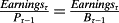
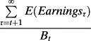
()Residual earnings, REτ = Earningsτ – iτ–1.Bτ–1, with iτ–1 the riskless spot rate. Price is thus given by Bτ and the (discounted) sequence of expected earnings and dividends (that imply expected book values). However, the dividend sequence is irrelevant to this valuation under M&M assumptions and accounting principles under which dividends do not affect the calculation of earnings but are paid out of book value (see Ohlson, 1995). Christensen and Feltham (2009) elaborate on this valuation.
 (2)
(2) is the discount rate for period τ given by the sequence of (one plus) periodic risk-adjusted expected returns from t + 1 to τ. Correspondingly, given clean surplus accounting,
 ()
()Residual earnings is now defined as REτ = Earningsτ – ERτ.Bτ-1, where ERτ is the expected return for period τ. A further expediency sets the expected return as a constant over time, but at some cost: if risk varies with the sequencing of earnings and its covariance with Ytτ, as in equation 1a, this feature is suppressed. Indeed, the notion of a constant discount rate is suspect from first principles; if the discount rate is time-varying, the assumption of a constant discount rate is inconsistent with the no-arbitrage assumption on which valuation theory is based, and one presumes that the discount rate varies with interest rates, risk preferences, the evolution of the firm, and (maybe) information in accounting reports. Ang and Liu (2004) demonstrate the valuation errors when time-varying discount rates are assumed to be constant.
Models (1a) and (2a) are the foundation of accounting-based valuation. However, apart from the clean surplus equation, not much has been put on the table. Importantly, the accounting for earnings and book value in these valuations is unspecified. As mentioned in the introduction, these models exhibit a value-irrelevance property with respect to the numerator accounting; the form of the accounting does not matter. However, the accounting also bears on the discount for risk, as the risk adjustment depends on the sequence of expected earnings and Ytτ. Accrual accounting generates that sequence, for it involves an allocation of earnings to periods, τ. Thus, the form of the accrual accounting is pertinent to the risk assessment. To stress the point, random numbers for earnings, with zero covariance with Ytτ, would have no implication for the risk discount. Just as the sequence of dividends and their covariance with Ytτ has no necessary bearing on value or the risk discount, so might the accounting without further specification.
A Framework to Evauate the Issues
 (3)
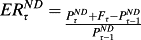
(3)- P1. Dividend irrelevance. Under M&M assumptions, dividends reduce price one-to-one, leaving cum-dividend returns unaffected. Correspondingly, dividends do not affect the RHS of equation 3 if
- (i) dividends do not affect contemporaneous earnings, and
- (ii) Pτ + dτ – (Bτ + dτ) = Pτ – Bτ.
- Earnings measurement induces a change in premium. Given P1,


-
An expected change in the premium implies expected earnings growth. If earnings are measured such that
 and thus Pτ – Bτ – (Pτ–1 – B τ–1) = 0, then,


That is, earnings are expected to grow at a rate equal to the (time-varying) expected return. 5 It follows that, if earnings are expected to grow at a rate different from the expected return, Pτ – Bτ – (Pτ–1 – B τ–1) ≠ 0, and Pτ – Bτ – (Pτ–1 – B τ–1) ≠ 0 implies expected earnings growth at a rate different from the expected return. See also Shroff (1995).
P1 grounds the analysis in no-arbitrage valuation theory. Under M&M, the expected return that reconciles successive price expectations (with no arbitrage) is insensitive to the timing of dividends, and P1 gives accounting conditions under which ERτ expressed in terms of accounting numbers exhibit this property. P2 brings the point on accounting measurement to the fore: the relationship between ERτ and accounting depends on how accounting is measured. P3 establishes a benchmark accounting where expected earnings equal expected returns (with no expected change in premium) and there can be no expected earnings growth beyond the ‘normal’ rate equal to the ERτ+1. More generally, earnings below this ‘normal’ earnings implies expected earnings growth with a corresponding increase in the premium. Put differently, Pτ–1 is based on the expectation of all subsequent (life-long) earnings, so the lower the expected period-τ component of those earnings, the higher must be the subsequent expected earnings relative to the period-τ earnings. Viewed in terms of the price-to-earnings (P/E) ratio, with no expected change in premium, ERτ =
 implies the expected forward P/E =
 , that is, a ‘normal’ P/E (without expected earnings growth). Accordingly, ERτ can be represented in terms of a sequence of expected earnings yields and price-denominated expectations of subsequent earnings growth.
However, if one is seeking information from the accounting that informs about the expected return, not much has been put on the table. Any measurement of earnings satisfies equation 3: a lower expected earnings yield, the first term on the RHS, merely implies an offsetting change in premium, with ERτ on the left-hand side (LHS) unaffected. Indeed, accrual accounting that determines the earnings in any one period can be arbitrary, without economic substance. Equation 3 is, after all, a tautology. CSR (alone) gives no resolution to the numerator issue or to the denominator issue; CSR just involves a substitution of earnings and book value for dividends, but ‘earnings’ and ‘book values’ are nothing more than names without more specification as to their measurement.
If the sequence of ERτ is to be informed by the accounting, one requires more structure on the accounting. That structure must communicate risk that results in a discount in the denominating price, Pτ–1 (and thus the current price, Pt) to yield a higher ERτ that reflects that risk. That is, the portion of expected life-long earnings to be recognized in period τ must communicate the ERτ for that period. That, again, is an accounting measurement issue, for accounting measurement is simply (!) an allocation of earnings to periods under specified accrual accounting principles.
Accounting for Risk and the Expected Return
We consider two alternative prescriptions for accounting for earnings and book values and examine how information about risk is conveyed under both.
Mark-to-market Accounting
Set Bτ = Pτ, all τ. Then, Pτ – Bτ – (Pτ–1 – B τ–1) = 0, and ERτ =
 by equation 3. Bt (current reported book value) is equal to the present value of expected cash flows, so imbeds both expected cash flows and the discount rate. Thus, like Pt to which it equates, Bt is not informative about the discount rate; the investor looks for information that informs about risk in Pτ, but Bt cannot supply it. Further, realized Earningst (equal to the cum-dividend change in book value) also conveys no information; earnings and price changes imbed revisions in both expected cash flows and future ERτ―so-called cash-flow news and discount-rate news―but not ERτ. Just as price changes convey little information about future ERτ, neither do earnings.
6And, the ERτ =
by equation 3. Bt (current reported book value) is equal to the present value of expected cash flows, so imbeds both expected cash flows and the discount rate. Thus, like Pt to which it equates, Bt is not informative about the discount rate; the investor looks for information that informs about risk in Pτ, but Bt cannot supply it. Further, realized Earningst (equal to the cum-dividend change in book value) also conveys no information; earnings and price changes imbed revisions in both expected cash flows and future ERτ―so-called cash-flow news and discount-rate news―but not ERτ. Just as price changes convey little information about future ERτ, neither do earnings.
6And, the ERτ =
 tautology remains: the expected earnings yield,
 = ERτ, but no information about ERτ is supplied by the accounting. In short, there is no accounting for risk and the expected return.
7
= ERτ, but no information about ERτ is supplied by the accounting. In short, there is no accounting for risk and the expected return.
7
These points are best demonstrated in the case of a marked-to-market bond. That accounting sets Pτ – Bτ – (Pτ–1 – B τ–1) = 0, and appropriately so, for a bond cannot have expected growth. Accordingly, ERτ =
 , with the earnings yield determined via the effective interest method. However, effective interest is inferred from the bond price and the bond yield it implies via an internal rate-of-return calculation. The accounting does not supply the expected earnings yield from which the ERτ can be inferred; rather it is the other way around.
While mark-to-market accounting (or fair value accounting) is somewhat hypothetical for equities―its application is quite limited in practice―it serves as a benchmark for examining accounting principles that depart from fair value accounting.
Mark-to-market Accounting for Financing Activities and Historical Cost Accounting for Operating Activities

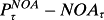
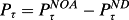
 is the price of the operating activities (enterprise price), NOAτ (net operating assets) is the book value of operating activities (enterprise book value), and
 and NDτ are the price and book value of the net debt, respectively. Marking net debt to market implies the following two properties:
-
Financing leverage does not affect the premium or the change in premium if net debt is marked to market: if
 , then Pτ – Bτ =
 .
.
 condition is not precisely met under GAAP, but is approximately so except when there is a significant change in interest rates or credit risk (and these changes are presumably close to zero in expectation).
-
Financing leverage impacts the expected return via the expected earnings yield. By the cash conservation equation of accounting, free cash flow (the net cash from operations), FCFτ = dτ + Fτ where Fτ is cash flow to net debtholders. As
 , ERτ can thus be expressed as

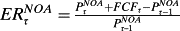 is the expected return for operations,
 is the expected return for net debt, and
 is the amount of leverage. This, of course, is the Modigliani and Miller (1958) leverage equation underlying the standard weighted-average cost-of-capital calculation.
 implies

 is the forward unlevered earnings yield and
 is the firm's net borrowing rate as reported in the financial statements (see Penman et al., 2015). Thus, leverage that increases the expected return to equity on the LHS of equation 3 also increases the expected earnings yield on the RHS of that equation. With no effect on the premium under P4, the leverage contribution to the expected return is captured via the earnings yield.
- Leverage increases expected earnings growth. By the same arithmetic for the expressions in P5,

Here is the insight: typically one views expected earnings growth as increasing price and thus decreasing the E/P ratio (increasing the P/E ratio). However, while leverage increases expected earnings growth, leverage has no effect on equity price under Modigliani and Miller's (1958) conditions. The growth from leverage that might otherwise add to price is risky growth so is discounted in the price; expected growth and risk cancel to leave the price unchanged. 8
And so, could it be that expected earnings growth associated with operating activities is also discounted in the price to yield a higher ERτ? If, like leverage, expected earnings growth is discounted because it is risky, that growth does not add to price. And, if the denominating price, Pτ–1, in equation 3 remains unchanged, ERτ will increase with the added numerator growth.
 (4)
(4) ()
()The standard view is that expected growth, g, adds to price and thus decreases the E/P ratio (and increases the P/E ratio). But, that is only so if ER is held constant while g varies. If ER increases with g, one for one, in equation 4a, then price does not change. The way this works with leverage has been demonstrated. With respect to operating activities, further information that connects growth to risk is needed. Can accounting supply that information?
- earnings are measured such that the expected growth generated by earnings measurement is at risk; and
- that risk is priced risk.
- The realization principle. Under uncertainty, GAAP and IFRS historical cost accounting defers the recognition of earnings until the uncertainty has largely been resolved.
Deferring earnings to the future reduces recognized earnings and, for a given Pτ–1, increases subsequent expected earnings, that is, it increases expected earnings growth. Further, under the principle, the earnings that are deferred are at risk, uncertain as to their realization. Correspondingly, realized earnings represent the outcome of the risk, risk resolved. Pt (current price) is the expectation of all future earnings but the timing of those earnings to periods, τ, is dictated by accrual accounting principles and the governing principle is the realization principle that is a reaction to uncertainty.
Indeed, under this principle, accounting can be seen as a system that tracks the resolution of uncertainty over time: earnings is recognized and book value added only when uncertainty is resolved, while the recognition of earnings still at risk is deferred to the future. Accordingly, the sequence of future ERτ in equation 3 can be represented as a sequence based on expected earnings realization but also earnings deferred. The deferral establishes prior probabilities for the Bayesian investor and realization revises those priors.
The deferral principle is applied with revenue recognition rules that (usually) require the firm to have a firm customer, with receipt of cash to be ‘reasonably certain’: expected future sales are not recognized, even though they may be anticipated in the price, because they are at risk of not being consummated. 10However, the uncertainty principle is also applied in expensing investments that are particularly risky―R&D, promotion, start-up costs, investment in software, distribution and supply chain development, employee training and retention, to name a few. 11This so-called conservative accounting reduces reported earnings but increases expected future earnings (from expected sales with no amortization of investment expenditure), that is, earnings growth. 12But the growth is risky: the payoff to the R&D etc. may not be realized. Feltham and Ohlson (1995) and Zhang (2000) recognize the property whereby conservative accounting depresses earnings and creates expected earnings growth, but with a constant discount rate. P7 opens up the prospect that this accounting may have implications for the discount rate; 13 Penman and Zhang (2015) elaborate. 14The accounting for earnings is path-dependent and the path depends on risk and its resolution.
It is far less clear whether condition (b) on the pricing of risk is satisfied. However, asset pricing theory demonstrates that it is satisfied for leverage: levered betas are higher than unlevered betas. Accordingly, the increase in expected earnings growth from leverage is at risk from market-wide shocks. Thus, it is not farfetched to imagine that shocks to expected earnings (growth) might be sensitive to economy-wide shocks such as shocks to GDP. The realization principle implies an effect on betas: in asset pricing terms, earnings are not recognized (and added to book value) until the firm can book a low-beta asset such as cash or a near-cash receivable; there is a different beta exposure with unrecognized earnings versus realized earnings.
Asset pricing theory (and valuation theory more generally) is built on the principle of no-arbitrage, and a no-arbitrage argument further supports the idea that the realization principle is tied to priced risk. In holding stocks, investors bear risk that the expected return may not be realized, and thus require a return commensurate with the risk. But, when they sell stocks and invest the cash proceeds in the risk-free asset―they realize the return―the risk is reduced, and so is the expected return (to the risk-free rate). A stock is a claim on the expected earnings of a firm, so when the firm realizes those expected earnings into cash or a near-cash asset on shareholders’ behalf, the investors’ risk and expected return are correspondingly reduced. On a consolidated basis, the firm's accounts are part of the shareholders’ accounts, so it makes no difference if the shareholder ‘realizes’ or the firm ‘realizes’ on the shareholder's behalf―the shareholders (the 100% owners) have the claim to the same cash. A no-arbitrage condition so dictates (frictions aside). The idea of realization as risk resolution also resonates with the economics underlying valuation theory: it is future consumption that is at risk in investing, and it is (realized) cash that buys consumption. Again, no-arbitrage applies: cash payout has no effect on cum-dividend value under M&M, so cash held in the firm has the same consumption value as cash on personal account. 15
These points aside, under asset pricing theory, condition (b) would require the risk that is recognized in the realization principle to be non-diversifiable risk. That is, the expected growth created under the principle would have to be growth that can be shocked by factors common to all stocks. (Of course, it remains an open question as to whether idiosyncratic risk is also priced.) One would love to have a property 8 that links the deferred earnings (growth) to priced risk and thus the expected return. That is too ambitious (for me) given we do not have a generally accepted asset pricing model for priced risk and return and, if we did, linking accounting operations to risk factors and their sensitivities is a challenging task. 16It would involve an identification of Ytτ and the covariance terms in model (1a) that discounts the sequence of expected earnings realizations.
However, there is evidence that suggests that this accounting conveys information about risk that is priced in the market.
Evidence
Penman and Reggiani (2013) show that average returns are related to the extent to which earnings are expected to be recognized in the short term versus the long term. Penman et al. (2015) show that portfolios with higher expected earnings growth are at a higher risk of that growth not being realized and that higher growth also has higher sensitivity to market-wide shocks to growth. Ellahie et al. (2014) report similar findings at the aggregate (country) level. Penman and Zhang (2015) find that firms where higher earnings growth is created by earnings deferrals under conservative accounting yield higher average stock returns. Correspondingly, expected earnings, so deferred, have higher variance around them and higher sensitivity to shocks to aggregate earnings. Based on P7, Penman and Yehuda (2015) extract a measure of the change in ERt from financial statements (‘discount-rate news’) and show that the market indeed prices this information as if it is news about expected returns.
All these results could be attributed to market inefficiency, of course. But that would be cavalier; the connection to risk via the realization principle cannot be dismissed lightly. The predicted returns in the papers just cited are not from data dredging with a search for t-statistics; rather the tests are structured with an understanding of how accounting connects to risk. That said, condition (b) remains an open question. That qualification must be kept in mind in reading what follows.
Implications for Existing Research
This analysis provides a commentary on a number of streams of accounting and finance research that attempt to connect risk and expected returns to accounting numbers. While the commentary is negative at points, it is provided in the spirit of improving the research. One requires a sense of balance: while points of theory should be recognized and implemented if possible, rough-and-ready approaches should not be dismissed out of hand if fine points are not operational.
The Implied Cost of Capital
 (5)
(5)The expected return, a constant called the ‘implied cost of capital’ (ICC), is then calculated as the internal rate of return that reconciles forecasts of forward earnings and a constant growth rate, g, to observed Pt – Bt. Variations include two or more years of forecasted earnings with a growth rate applied at the longer forecast horizons or (in Gebhardt et al., 2001) with an assumption that book rates of return will decline to an industry benchmark over time. Other papers, such as Gode and Mohanram (2003), reverse engineer the Ohlson-Juettner (2005) model with a constant growth rate. See Easton (2007) and Easton and Monahan (2016) for a review and commentary. Note that, as this expected return is inferred from price, it cannot be inserted in model (2a) to calculate price. For that, one needs (accounting) information that is independent of price.
Some papers have shown that ICC measures are somewhat related to conjectured risk measures such as beta, leverage, and industry membership, in Gebhardt et al. (2001) and Botosan and Plumlee (2005), for example. However, the research has been largely unsuccessful in predicting average returns, a failure in validation. Guay et al. (2011) and Easton and Monahan (2005) discuss. This state of affairs is quite remarkable given that many accounting numbers (with less pretense to being the expected return) readily predict returns (and robustly so), for example, E/P, B/P, accruals, growth in assets, and a number of financing variables, to name a few. This predictive ability could be attributed to market inefficiency, but the ICC is the implied internal rate of return implicit in the current price so should similarly identify market mispricing. The problem is more likely to be in the approach and/or the inputs. Much is at stake; a considerable amount of research on disclosure, earnings quality, audit quality, regulatory institutions, and corporate governance mechanisms rides on the effect of these features on the ‘cost of capital’ as measured by the ICC. This research seems to have taken on a life of its own with broad acceptance that ICC measures the cost of capital.
Much of the critique of ICC estimates focuses on using analysts’ forecasts as an input. The Lewellen (2010) critique stresses this issue, among others. Mohanram and Gode (2013) and Wang (2013) demonstrate some improvement in dealing with it. Other papers such as Hou et al. (2012) and Li and Mohanram (2014) replace analysts’ forecasts with forecasts estimated from accounting data, with some success. Lee et al. (2014) propose a framework for evaluating alternative ICC estimates. The review below focuses on the approach rather than the inputs.
First, the assumption of a constant expected return (and estimating the cost of capital) based on forecasted earnings is doubtful if ERτ varies with the expected time-varying realization of earnings as uncertainty is resolved. For example, if ERτ is time-varying, the ICC estimated with the input of a long-term earnings growth rate, g, may be a poor predictor of short-term expected returns, perhaps explaining the inability of ICC estimates to forecast year-ahead returns. 17
Second, the typical assumption of the same growth path for all firms is likely to be violated; indeed, estimating different growth rates over firms, as in Nekrasov and Ogneva (2011), shows improvement in predicting returns. This point is well recognized, but our analysis adds a further dimension: if expected growth is connected to risk and the expected return under the realization principle, ER and g in model (5) are connected, a higher g implies a higher ER. Failure to distinguish different growth rates across firms may thus fail to distinguish different risk. And failure to input a growth rate commensurate with the indicated risk confounds the ICC estimate. Further, the joint estimation of ER and g in Easton et al. (2002) as if they were independent inputs to a valuation is suspect if growth is risk. The connection of growth, risk, and the expected return in P5 and P6 makes the point: leverage increases both expected earnings growth and risk, and also ERτ. The realization principle suggests that this might also apply to operations.
Cash-flow Betas
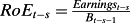
A number of papers have attempted to calculate so-called ‘cash-flow betas’. See Cohen et al. (2009), Campbell et al. (2010), and Nekrasov and Shroff (2009), for example. The labelling is confusing because these ‘fundamental betas’ are actually estimated slope coefficients from regressions of firm return on equity (ROE) on market-wide ROE, not cash flows. The estimation is an admirable attempt to come to grips with the covariance term in model (1a).
However, there are accounting issues that frustrate the endeavour. In the inter-temporal Merton (1973) asset pricing model, investment opportunities are linked to the state of the economy.
18Under conservative accounting, earnings in the numerator of ROE are reduced with growth in risky investment. If firms increase that investment in good times when market-wide ROE is up, they will reduce the firm ROE, inducing a negative correlation between ROE and market-wide ROE (and thus will appear to have lower rather than higher risk). Similarly, firms may reduce investment in bad times, increasing ROE when market-wide ROE is down. Conservative accounting, with its generation of risky expected growth, signals higher risk, but induces a lower correlation between ROE and market-wide ROE. There is also the issue of estimating one covariance over periods where discount rates may vary and the composition of deferred and realized earnings differs from period to period to indicate those changing discount rates. With reference to P3, cash-flow beta estimates are appropriate with constant premiums over time (no growth). In that case ERτ =
 , all τ.
19
, all τ.
19
Applications of the Vuolteenaho (2002) Model
A string of papers embrace the Vuolteenaho (2002) model to decompose stock returns into components that are attributed to expected returns, cash flow news, and expected return news and to connect accounting numbers to each component; see Callen and Segal (2004) among others. The model is implemented in a vector autoregressive (VAR) scheme to estimate the linear dependencies in the time series evolution of indicator variables and returns and, in turn, to identify the three return components from residuals from the modelling. In Lyle and Wang (2015) and Chattopadyhay et al. (2015), the model is applied to estimate the expected return from accounting data as an alternative to ICC calculations, and with success in predicting returns out of sample. Unlike the analysis in this paper, the modelling has the appealing feature of explicitly connecting accounting numbers to the expected return and its variation. The Callen (2016) paper in this issue lays out the scheme and supplies references to papers that employ it. Easton and Monahan (2005, 2016) evoke the model in evaluating ICC estimates.
Like equation 3, the clean surplus relation is evoked to state the Voulteenaho tautology, tying ROE and B/P to the expected return. However, an additional assumption is implicit in the auto-regressive modelling. In some papers, log(Pτ) – log(Bτ) is assumed to converge to zero in the long run. And/or, ROE is assumed to evolve according to an autoregressive parameter to equal the expected (stock) return, ERτ in the long run. Chattopadyhay et al. (2015) allow for the expectation Pτ – Bτ to be non-zero but constant in the long run. However, they maintain the autoregressive assumption such that growth in book value and market value converge linearly to zero over time and ROE is anchored on the long-run expected return. Lyle et al. (2013) also model the evolution of (residual) earnings with an autoregressive assumption to estimate expected returns.
Modelling the evolution of log premiums is curious for, unlike Pτ – Bτ, log premiums are affected by dividends, so P1 (and M&M) are violated. 20But, further, P2 demonstrates that the evolution of the premium, Pτ – Bτ, is dictated by the accounting for earnings, and the autoregressive assumption for the evolution of this premium imbeds a specific accounting. If Pτ – Bτ = 0 in expectation, we have the ‘unbiased accounting’ of Ohlson (1995). The assumption might be modified such that Pτ – Bτ > 0 in the long run, but the path to the long run is critical. P3 shows that expected earnings growth implies an expansion of premiums: Pτ − Bτ – (Pτ–1 − Bτ–1) > 0. So, for the typical case of Pt – Bt > 0, an autoregressive assumption where the premium declines (linearly) over all τ, does not admit earnings growth that implies an increase in premiums, nor does it accommodate the conservative accounting of P7 that yields that growth, so pervasive in GAAP and IFRS. In short, the modelling does not admit a path-dependent evolution of earnings tied to risk resolution.
The Ohlson (1995) paper with unbiased accounting was supplemented with the Feltham and Ohlson (1995) paper with ‘biased accounting’ under which Pτ – Bτ > 0 in expectation, all τ, and the (conservative) accounting involved can yield expected growth (and, correspondingly, an expansion of price premiums over book value). See also Zhang (2000). Under that accounting, ROE does not correspond to the expected return in expectation. The growth (and increasing premium) generated by conservative accounting reduces earnings in the numerator of ROE such that ROE increases (to a level well in excess of the expected return) as the firm matures with subsequent realization of the deferred earnings (and then only if the risk pays off). Consider Microsoft, Apple, Google, and Infosys, mature firms with high ROE (and, more so, RNOA), compared to a new firm, Twitter, with a low ROE due to expensing investments but similarly a low B/M. The anchoring of expected ROE to the expected return is justified as driven by ‘the forces of competition’, and the reversion of ROE to that ‘normal’ return under an assumed AR(1) parameter is said to reflect the speed at which those forces erode profitability. But that is economic modelling, as if book rate of return were ‘real profitability’. 21 Rather, ROE is an accounting measure driven by the realization principle and conservative accounting. There is nothing in that accounting that anchors ROE to the expected return in expectation (although boundary conditions must be met). On the contrary, rather than a high ROE indicating higher risk and expected return, with both declining over time, the accounting indicates that a lower ROE affected by conservative accounting indicates a higher risk, with risk and the expected return declining as ROE increases with earnings realizations.
Penman and Zhang (2015) elaborate and present supporting evidence based on an analysis of the actual accounting rather than an assumed parameter for the dynamics. Based on the realization principle, Penman and Yehuda (2015) extract measures of discount rate news directly from financial statements that look quite different from those estimated via the Vuolteenaho model. The measures satisfy a set of validation tests; in contrast, the discount rate news and cash flow news component of returns estimated with the autoregressive scheme fail consistency requirements that must be satisfied for such news.
On a more general level, both theory and empirical papers often assume a ‘process’ for the evolution of earnings―an AR(1) process is common. Papers on the time-series properties of earnings, earnings persistence, as well as those that connect accounting numbers to prices come to mind. But an assumed process implies an assumption about accounting principles for recognizing earnings over time, and that implied assumption may not be appropriate if the model is applied to GAAP or IFRS data generated under different accounting principles.
One might well ask, given the critique here, why estimates of the expected return from the Voulteenaho model predict actual returns out of sample. That raises another issue.
ROE, Risk, and the Expected Return
In the Vuolteenaho model, ROE surfaces as an indicator of expected returns, with a higher ROE indicating higher returns, ceteris paribus. More generally, ROE and similar measures of profitability have been shown to be positively related to returns, in Novy-Marx (2012) and Ball et al. (2015), for example. The explanation offered rests on the standard risk return tradeoff: higher risk requires higher returns, so the positive association between ROE and returns is because higher ROE is the reward for taking on risk. The applications of the Vuolteenaho model formalize this intuition by anchoring ROE to the expected return. Apparently in response to these observations, Fama and French (2015) have developed a ‘five-factor model’ that adds a measure of ROE to other factors to explain stock returns.
However, in these papers, book-to-market (B/P) is included in the ceteris paribus condition, so the positive relationship between ROE and returns is conditional on B/P. But, E/P = E/B × B/P = ROE × B/P, so adding ROE to a predictive regression that also includes B/P recovers E/P, and E/P is the first term that connects accounting numbers to the expected return in equation 3. Indeed, in the no-growth case (with no change in premiums), ERτ is equal to the forward earnings yield, so one would expect ROE and B/P to predict returns (jointly) in this case if current ROE is a good indicator of forward ROE (which it is). But this is not because ROE is an indicator of risk and return but because ROE, in combination with B/P, yields E/P that indicates risk and return (in the no-growth case).
However, the no-growth case is not typically for equities so the specification is not complete without an indicator of growth that connects to risk. Equation 3 indicates that the appropriate specification is to include E/P and then add variables that indicate risky expected earnings growth. B/P is identified as such a variable, in Penman et al. (2015). If ROE were positively related to expected returns, it would have to be that, conditional on E/P, ROE also indicates risky growth. However, under the accounting principles in P7, growth is induced with lower current earnings due to earnings deferrals, and lower earnings imply lower ROE (via the numerator). Thus a lower ROE, rather than a higher ROE, indicates risk and a higher expected return if the risk indicated by the accounting is priced risk. The tests in Penman and Zhang (2015) provide support: unconditionally, there is no relation between ROE and returns but, conditional on E/P, ROE robustly predicts returns negatively, with the relationship considerably stronger for ROE that are affected by conservative accounting. Further, the (deferred) earnings predicted by ROE are at a higher risk of not being realized and are particularly sensitive to market-wide shocks to earnings.
Fama and French Connection of Discount Rates to Accounting Numbers

 , as profitability (rate of return on book value), and the change in book value,
 , as growth in investment. Reverse-engineering the expression, they conclude that r is increasing in B/P, holding the expected book rate of return and expected investment growth constant, increasing in the expected book rate of return holding B/P and expected investment growth constant, and decreasing in expected investment growth holding B/P and expected book rate of return constant. These comparative statics motivate the five-factor model in Fama and French (2015).
However, the comparative statics are inconsistent with how accounting works. For a given price, one cannot vary B/P while holding book rate of return (profitability) constant, because both reflect the accounting for book value. High book rate of return means low B/P, ceteris paribus, by construction of the accounting. As indicated immediately above, this is strictly so in the case of no growth: r = E/P, by equation 3 and E/P = E/B × B/P (where E/B is profitability). Thus, the expected return is given by E/P rather than B/P and E/B as separate inputs. Indeed, B/P and E/B can be any value (but the mirror image of each other because of the common effect of the accounting for book value), yet still yield the same E/P. The same critique applies to the claim that r is increasing in profitability holding B/P constant (as discussed above). On the connection of ‘investment’ to the expected return, there is a mislabelling that voids the interpretation: growth in book value in the formula is not investment. Rather, Bτ – Bτ–1 = Earningsτ + dτ. Thus, as dividends are not relevant under P1, growth in book value is driven by earnings and the profitability that involves those earnings. So, profitability cannot be held constant while looking at the effect of growth in book value on r.
The Fama and French comparative statics appear to support the view, standard in asset pricing, that expected returns are negatively related to growth―as in the standard ‘value’ versus ‘growth’ spread where ‘growth’ yields lower returns than ‘value’. In contrast, P7 suggests that the expected return is positively related to growth. The Fama and French formulation does not admit the period-to-period growth envisioned in P7. With the infinite summation over expected future earnings in their model, the earnings expectation relative to current book value is for life-long earnings, with no allocation to periods. In contrast, P7 focuses on the allocation of earnings to the short-term versus the long-term that introduces expected earnings growth. The ‘value’ and ‘growth’ labels do not stand up to scrutiny, as explained in Penman and Reggiani (2014).
A Re-Think Of anomalies Research
Considerable empirical research connects accounting numbers to average stock returns, among them E/P, B/P, accruals, investment, growth in assets, and a number of financing variables. In asset pricing research, the tendency has been to attribute these ‘anomalies’ to risk and expected return, while accounting research tends to attribute them to mispricing. In the absence of a validated, generally accepted asset pricing model, the attribution will not be resolved, but the introduction of the realization principle as the driver behind accounting numbers requires a re-think on the part of those who ascribe returns that are predicted by accounting numbers to abnormal returns.
Consider three very popular ‘anomalies’: accruals, investment, and growth in net operating assets (ΔNOA).
22Under P4, a change in premium is explained by ΔNOAτ, the accounting for operating activities: if
 , Δ(Pτ – Bτ) = Δ
 – ΔNOAτ. Accordingly, expected earnings growth that induces the change in premium is determined by the accounting for NOA.
23If that growth is connected to priced risk, then the ΔNOA anomaly is explained: higher (lower) ΔNOA implies lower (higher) expected growth and correspondingly lower (higher) risk and average returns, as observed. And, as ΔNOA = Investment + Other Accruals (a fixed accounting relation), then the investment and accrual anomalies are similarly explained. High accruals are associated with lower returns, but high accrued earnings come from realized earnings (driven by the sales accounts receivable accrual and expense matching), and realized earnings imply the resolution of risk and lower expected returns. Investment opportunities are at risk, and that risk is priced under a Merton inter-temporal asset pricing model. Realization of investment and booking it to the balance sheet is the resolution of that risk, so yields lower returns, as observed. However, conservative accounting also operates: if the investment is deemed too risky, the investment is expensed immediately, yielding lower ΔNOA ceteris paribus and expected earnings growth. If that growth is risky, the conservative accounting (that is a response to risk) should be associated with higher average returns, as observed in Penman and Zhang (2015).
– ΔNOAτ. Accordingly, expected earnings growth that induces the change in premium is determined by the accounting for NOA.
23If that growth is connected to priced risk, then the ΔNOA anomaly is explained: higher (lower) ΔNOA implies lower (higher) expected growth and correspondingly lower (higher) risk and average returns, as observed. And, as ΔNOA = Investment + Other Accruals (a fixed accounting relation), then the investment and accrual anomalies are similarly explained. High accruals are associated with lower returns, but high accrued earnings come from realized earnings (driven by the sales accounts receivable accrual and expense matching), and realized earnings imply the resolution of risk and lower expected returns. Investment opportunities are at risk, and that risk is priced under a Merton inter-temporal asset pricing model. Realization of investment and booking it to the balance sheet is the resolution of that risk, so yields lower returns, as observed. However, conservative accounting also operates: if the investment is deemed too risky, the investment is expensed immediately, yielding lower ΔNOA ceteris paribus and expected earnings growth. If that growth is risky, the conservative accounting (that is a response to risk) should be associated with higher average returns, as observed in Penman and Zhang (2015).
In short, these anomalies are consistent with rational pricing if the realization principle aligns with the evolution of risk and the expected return. The evidence in Penman and Zhu (2014) suggests so.
The Numerator Issue
As indicated in the introduction to the paper, practical valuation requires not only information about the discount rate, the denominator issue, but also the specification of the accounting for the numerator. The residual income model, based solely on the clean surplus relation, is agnostic about the numerator issue. However, the analysis that deals with the denominator issue also directs the accounting for the numerator; a discount rate for any period, τ, must refer to the risk that the expected payoff for that τ may not eventuate.
The residual income models in equations 1a and 2a require (1) a division of the value in Pt between Bt and expected earnings not yet recognized and (2) the allocation of those total earnings not yet recognized to each future period, τ. Both issues concern the allocation of earnings to periods―the present versus the future and inter-temporally (in expectation) in the future.
Book value is not discounted in the model, so must involve numbers that do not have to be discounted for risk. As Bt is accumulated earnings recognized to date net of accumulated net dividends (that include net share issues), our analysis suggests that those earnings in book value are realized earnings where the uncertainty about outcomes has been resolved. Assets are added to the balance sheet only at cost (with no added value for the expected earnings that might accrue). If, ex post, expected earnings imply carrying values higher than the value in those earnings, the balance sheet is written down. Further, if the outcome to the investment is highly uncertain, conservatism applies such that the asset is expensed and not put on the balance sheet. This accounting, along with the recognition of operating liabilities, yields a balance sheet that will only be affected if earnings are realized in the future, and a balance sheet that has low probability (ex ante) of being written down. On point (2), the identification of expected earnings to each τ is based on the timing of their expected realization such that they are sequenced with the τ indexed covariance term in model (1a) that discounts for the risk that earnings realization may be affected by common shocks.
With this accounting, the residual income model is now really an ‘accounting-based valuation model’. It has the feature of accommodating risk and the feature of anchoring a valuation on a book value that contains little risk apart from leverage transparently reported on the balance sheet; there is nothing in the balance sheet that can come back and hit you later―no ‘water in the balance sheet’ as a fundamentalist would say. And it has the feature of identifying where the risk of the business lies―the risk of earnings not being realized.
Accounting Policy
If accounting is to serve the investor, these points have implications for accounting policy, a topic in which Abacus has shown a keen interest over the years. There are also implications for the current debate about fair value accounting versus historical cost accounting. Fair value accounting is said to be more timely, for it projects future cash flows, while historical cost recognizes the information in price with a lag. However, in the comparison of the two accounting measurements earlier, historical cost accounting conveys the risk in investing while fair value accounting fails to do so. In fact, fair value accounting (even if ideally implemented) does not project future cash flows but rather the (discounted) present value of expected cash flow. As anyone carrying out practical valuations knows, the identification of the discount rate is problematical, but the information about risk that might supply this aspect of fair value accounting would be lost with fair value accounting. While other issues enter the debate, this is one to consider.
This raises the prospect that ‘good accounting’ is less timely accounting, in contrast to the standard view that accounting is deficient for not being timely. Accounting that recognizes the earnings expectations in price with a lag informs the investor of that delay it tied to risk and its resolution. Research has typically seen accounting as providing information about expected cash flows―cash flow news―but the investor also requires discount rate news. After all, equity value is based, not only on expected cash flows but also on the rate at which the cash flows are to be discounted. Indeed, the objectives in the Conceptual Framework of the IASB and FASB state that accounting information should provide investors with information to assess ‘the amount, timing, and uncertainty of future net cash flows’. Historical cost accounting with a realization principle tied to the resolution of uncertainty satisfies the objective.
Earnings recognition under historical cost accounting is often presented as a matter of recognizing revenue under the realization principle and then matching associated expenses against the revenue to determine the earnings. That matching involves holding costs on the balance sheet then taking them to the income statement under an amortization rule. Conservative accounting that expenses investment costs immediately violates matching, bringing calls for the ‘intangible assets’ so expensed to be capitalized and amortized. However, the analysis here suggests that the mismatching with conservative accounting conveys information about risk and its resolution that would be lost with such capitalization of risky investments. This accounting accords with the FASB's Statement of Financial Accounting Concepts No. 2 (1975), which defines conservative accounting as ‘a prudent reaction to uncertainty’. 24In justifying the immediate expensing of R&D under FASB Statement No. 2, the FASB focused on the ‘uncertainty of future benefits’. In IAS 38, the IASB applied the criterion of ‘probable future economic benefits’ to distinguish between ‘research’ (which is expensed) and ‘development’ (which is capitalized and amortized). An understanding of conservative accounting suggests the ‘matching principle’ should not be embraced as a matter of accounting principle if one wishes to convey information about the amount and uncertainty of future cash flows.
In fact, mismatching is inevitable and the policy question is how to design the mismatching. Matching is an operation that can only be implemented under certainty: if one knows both the amount and timing of future revenues, one can match expenses with those revenues perfectly, but even then only if the association of expenses with revenues can be identified. Under uncertainty, the accountant is faced with a choice between capitalizing risky investment with an uncertain amortization rate to achieve the matching or expensing it immediately. In both cases, the settling up against the accounting comes with the resolution of uncertainty. If investment is capitalized and revenues fail to materialize, mismatching occurs ex post with write-offs of carrying values against revenues to which the impairment does not apply. Implicitly, the write-offs recognize that, on an ex post basis, assets have been inappropriately recognized on the balance sheet. With the expensing of risky investments, mismatching is implemented immediately but with the risk now communicated ex ante. So the policy question is whether the accounting should communicate risk ex ante or ex post. Prudent (conservative) accounting would suggest the former. Fair value accounting is a third alternative, again with risk communicated (too late) ex post as fair values are shocked when it is recognized that expected earnings built into the fair value will not materialize. 25
Discounted Earnings
The task of identifying the economy-wide Ytτ variable and the covariance term in model (1a) is challenging, as research in asset pricing has found. Enhanced valuation models add further structure to interpret Ytτ; for example, in consumption-based models it represents investors’ marginal utility of consumption at τ relative to time t, which (with further assumptions) is couched in terms of aggregate consumption. As a matter of measurement this is problematic, and thus the recourse to the practical expedient of model (2a). However, calculating a risk premium for the discount rate remains a challenge, one that has been pursued relentlessly in asset pricing.
But a tantalizing idea surfaces: what if accounting could be designed with an earnings calculation,
 = REτ – Cov(REτ, Ytτ)? That is, the discount for risk in the numerator of model (1a) is built into the earnings measurement (such that expected earnings require no discount for risk). The realization principle and conservative accounting appear to imbed this feature: in the presence of risk, earnings are reduced―discounted for the risk―and deferred contingently to the future. If the deferred earnings are realized with risk resolution, the recognized earnings indicate lower risk. It is not clear whether an accounting could be calibrated that captures the risk but given the difficulty of the alternative―identifying Ytτ and covariances―the idea is worthy of consideration.
In any case, the following conjecture is on the table: if GAAP or IFRS already discounts earnings for risk, the covariance discount that is directed by model (1a) may be redundant, at least to some extent. If we see a company with earnings prospects but with current earnings depressed by conservative accounting, is that not a risky company? Amazon and Twitter look like that sort of firm. They presumably have high earnings expectations but have low or negative earnings and low ROE from the expensing of investments (as of the date of writing). The accounting informs that the expected earnings are at risk, they may not materialize. On the other hand, Coca-Cola reports a high ROE in the order of 25% because the investment in promoting its brand has paid off with realized earnings; it has a beta of 0.4.
References
- 1 Demirakos et al. (2004), Hand et al. (2015), and Pinto et al. (2015) survey the use of valuation models in practice.
- 2 This is understood when it is claimed (correctly) that discounted cash flow valuation (cash accounting) and accrual-accounting residual income valuation converge with infinite forecasting horizons.
- 3 Penman (1997, 2015) demonstrates how accounting affects valuation and its errors with finite-horizon forecasting.
- 4 This identity has long been recognized for realized returns, for example in Easton et al. (1992). We adapt it here to apply to expected returns.
- 5 If Earningsτ = Earningst+1, all τ, the accounting is sometimes referred to as ‘permanent income accounting’ whereby Earningst+1 is sufficient for forecasting all future earnings. One can show that, if Earningsτ = Earningst+1, all τ, then ERτ = ERt+1, all τ, that is, the expected return is constant over time. Setting dτ = 0 is for simplicity; dτ ≠ 0 reduces Earningsτ+1, but, with the dividends reinvested at the rate, ERτ+1, cum-dividend earnings are unaffected, given P1.
- 6 Just as one might infer the expected return from a (long) time series of shocks to prices, so might one do so from shocks to book values (earnings) under mark-to-market accounting, provided that the expected return were a constant over that observation period. But this is doubtful with changing discount rates where shocks reflect both cash-flow news and discount-rate news.
- 7 Cochrane (2011) makes the same point about fair value accounting.
- 8 Penman (2013, Chapter 14) provides numerical examples.
- 9 The full payout assumption is unimportant. Payout (retention) other than full payout adds to earnings growth, g, but does not add value under M&M conditions, nor does it affect the premium of price over book value under P1. The valuation in equation 4 isolates the growth that potentially affects price and the expected return, r, and at the same time is M&M consistent. Penman et al. (2015) connect growth to the expected return via the Ohlson and Juettner-Nauroth (2005) model that generalizes the Gordon model by maintaining M&M properties for all payouts.
- 10 New IASB and FASB proposals for revenue recognition require satisfaction of a contract, and contract resolution appears to have the feature of removing uncertainty.
- 11 Kovacs et al. (2015) estimate that, on average, a third of selling, general and administrative expenses in US financial statements have investment characteristics.
- 12 ‘Conservative accounting’ is characterized in different ways in the literature. It is used here to mean any accounting that results in price greater than book value, which, in turn, implies that expected earnings in price are recognized (and added to book value) with a delay.
- 13 A special case involves conservative accounting for investment with no change in the premium: if there is no growth in investment, earnings (and the premium) are not affected, even though conservative accounting is applied to the investment. So, for example, earnings are not affected by the expensing of R&D if there is no growth in R&D; in steady state, earnings are the same whether R&D is expensed immediately or capitalized and amortized. With respect to risk, this steady-state property―the so-called cancelling error property of accounting―occurs when the reduction of earnings from expensing new risky investment is exactly offset by the realization of earnings from earlier investments.
- 14 Penman et al. (2015) demonstrate many of the properties in this section with examples, including a case where expected growth is priced to yield a higher expected return.
- 15 Realization typically results in a receivable rather than cash, but receivables are discounted to a cash equivalent value for the risk of not receiving the cash, at least in principle.
- 16 Ohlson (2008) lays out a model where permanent income accounting with a constant expected return (as defined in P3) is modified to yield a constant growth rate that equates to the risk premium (and, in turn, implies an expected increase in premiums of price over book value). The paper envisions an allocation of life-long expected earnings to periods with this feature, but is silent on the transaction analysis and accrual accounting principles that could induce earnings growth that is tied to risk.
- 17 This point complements the criticism of Hughes et al. (2009) that, with time-varying expected returns, the internal rate of return is not the expected return.
- 18 Also, under Cochrane's (1991) Q-theory, firms invest in good states when discount rates are low.
- 19 Equation 3
 and is covariance with the market earnings yield, rather than ROE, as the way to estimate “cash flow betas”.
 - 20 This is more than just a passing comment. Modelling that violates a foundational principle of modern finance is called into question unless it is justified by a relaxation of one of the assumptions in M&M.
- 21 An AR(1) assumption is also sometimes justified by the empirical observation that ROE is mean reverting, as in standard profitability ‘fade diagrams’. But the empirical documentation refers to the evolution of past (realized)
 which is not the same as
 , by Jensen's inequality.
 - 22 The original papers appear to be Sloan (1996), Titman et al. (2004), and Fairfield et al. (2003), respectively.
- 23 P2 ascribes the premium to the measurement of earnings. As financing does not affect premiums, that measurement pertains to operating income (OI). As OI = Free Cash Flow + ΔNOA by the clean surplus relation for operating activities, the measurement of earnings is determined by ΔNOA. (Correspondingly, it can be shown that free cash flow does not affect premiums.)
- 24 The 2010 and 2015 IASB Discussion Papers on the Conceptual Framework dispense with the notion of conservatism in favour of ‘neutrality’ and define prudence as ‘caution when making judgments under conditions of uncertainty’.
- 25 Barker and Penman (2015) invoke these ideas to address the recognition and measurement issues in the proposed Conceptual Framework of the IASB.