Endogeneity in Accounting and Finance Research: Natural Experiments as a State-of-the-Art Solution

Endogeneity is more than a problem of econometrics. It is also a problem of theory. The issue for researchers is that often variables included in the structural equations are simultaneously determined, mismeasured and/or the theory is incomplete and so important variables are omitted. More sophisticated econometric techniques are only part of the solution. Better theory is also necessary to help researchers build more complete and accurately specified models.

In finance and accounting research it is important that empirical work is underpinned by theory. Accordingly a well-designed study must be clear about how and why variables influence one another and the logic and direction of the relationship must be specified (Larcker and Rusticus, 2007). However, much of the accounting and finance empirical literature is plagued by endogeneity, particularly in corporate governance studies (Roberts and Whited, 2012). A spate of recent articles addressing the concerns of endogeneity in the finance and accounting literature is putting this issue firmly on the table. For example, Chenhall and Moers (2007), Larcker and Rusticus (2007), and Van Lent (2007) in accounting. And in finance, Roberts and Whited (2012) and Brown et al. (2011). Endogeneity has always been present and recognized as a problem that undermines causal inference. However, it is often a problem that researchers either do not address at all, or simply note in passing that the problem exists. Table 1 selects the papers with endogeneity issues published in 2013 and 2014 in Asian Pacific journals including: Australian Journal of Management (9), Accounting and Finance (11), Abacus (1), Pacific Basin Finance Journal (2), and International Review of Finance (1). Out of the 24 papers listed in the table, only two performed all specification tests and more than half (13) performed no tests.

Ignoring the problem, however, does not mitigate the implications—endogeneity limits the validity of empirical testing of models. Here, we do not question the validity of finance and accounting research to date to the extent that it should be disregarded. We argue that endogeneity has become more of a concern as we model increasingly complex relationships. Accordingly, the power of our theories is more keenly scrutinized and tested.

While all agree the problem is pervasive there is some disagreement about how best to deal with it. Chenhall and Moers (2007) and Larcker and Rusticus (2007) argue that theory development is critical. Van Lent (2007) on the other hand, argues that theory is never likely to be complete and good instruments are hard to find and so there is little a researcher can do to mitigate endogeneity. He argues that good research should be judged by how stimulating the research question is and it is a mistake to pretend that models are fully specified. Researchers should rather defend why they chose that particular misspecification and articulate how the results would change had they chosen another misspecification of the model. Roberts and Whited (2012) emphasize the importance of researchers discussing endogeneity along with good empirical design using high-quality data and robust testing of empirical predictions. Researchers should not be discouraged from empirical testing because even if endogeneity is known to be present, such studies provide the foundation for future work (Roberts and Whited, 2012).

Where researchers recognize endogeneity as a limitation to their research, how they deal with it is constrained by current thinking on appropriate techniques. Commonly used research designs to deal with endogeneity include two-stage least squares (2SLS), instrumental variables (IV), differenced GMM (generalized method of moments), and system GMM as we can see from Table 1. In the next section we provide a unifying framework that illustrates and encompasses all of these approaches.

Looking beyond the textbook solutions, one research design that helps mitigate the problem of endogeneity is that utilizing a natural experiment. A study incorporating a natural experiment provides the researcher leverage over the commonly used textbook solutions to endogeneity because it involves making use of a plausibly exogenous source of variation in the independent variables of interest (Meyer, 1995). If the naturally occurring event is convincingly exogenous, and the study well implemented, then researchers have a way to isolate causal links, build new theory and clarify (confirm/disconfirm) existing theory by mitigating the issue of endogeneity. In this paper, we provide researchers with a road map for designing research based on natural experiments and in this way we contribute to the evolution of more rigorous research techniques in finance and accounting.

Endogeneity and Current Textbook Solutions

The current textbook solutions to endogeneity include 2SLS, IV, differenced GMM, and system GMM.1 In the section that follows, we work through these methods and provide a unified framework showing how these approaches are related.

Errors in Variables Problem

To understand endogeneity we can first liken it to the errors in variables problem. The following greatly simplifies this problem. Let's define the relationship:

where: X = X* + ε

i.e., X* = True value and X measures X* with error

This implies that the X variable is not independent of the error and that omitted variables, which may be variables we are unaware of or simply cannot be quantified, are correlated with the error term.

Ordinary least squares (OLS) minimizes the sum of the squared errors:

This has the following first-order conditions known as the normal equations of OLS:

()

()

We will show in this section that all of the econometric methods to address endogeneity can be thought of in terms of these normal equations of OLS. They will be the basis for moment conditions that define the GMM estimators. The approach will nest the maximum likelihood approach with the advantage that the coefficients and standard errors will be the same if the maximum likelihood assumptions are correct but that the standard errors of the GMM approach will be valid whether or not the maximum likelihood assumptions are correct. Solving the normal equations of OLS—equations 1 and 2 above—yields the normal β estimate:

Since X is measured with error: X = X* + ε

Hence, the calculated Beta is a biased and inconsistent estimator of the true Beta. This comes about because the X variable is not independent of the error term.

Two-stage Least Squares (2SLS), Instrumental Variable (IV)

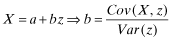
The standard solution to the errors in variable problem is to use an IV z, which is (1) not correlated with the error term ε (i.e., exogenous) and (2) is relevant to X* (i.e., non-zero correlation).

The IV estimator is:

We can think of this as a two-stage procedure:

Stage 1: Run the regression
Now define the instrument to be:
Stage 2: Run the regression

This implies that:

Now substitute:

from the first stage regression and we have:

We can see that 2SLS gives us the familiar measurement error IV estimator.

Now we will show how 2SLS and IV estimators can be thought of in a general GMM framework. Think of the normal equations of OLS (equations 1 and 2 above):

Solving for β we obtain:

If we replace X with z in the 2^nd equation:

This implies that the instrumental variable estimator. We will show how the GMM moment conditions based on the normal equations of OLS, that is, equations 1 and 2, will nest all of the endogeneity estimators.

The GMM moment conditions based on the normal equations of OLS gives us another way to think of the IV estimator. Take the following example:

The simultaneous equations are:

()

()

where the Ys are endogenous variables and the Xs are exogenous variables. The problem is similar to the measurement error issue, that is, where Y is correlated with μ. This can be seen from equation 4 where Y₂ contains the error term μ₂, which then induces in equation 3 a problem similar to measurement error and with similar consequences, that is, biased and inconsistent estimators.

Now consider estimating (3) with 2SLS:

• (1) 1^st stage:

  Regress Y₂ on the exogenous variables:

  

Now define the instrument as:

• (2) 2^nd stage:

  In the regression for Y₁ use the instrument instead of Y₂ as follows:

  

Now consider estimating (4) with 2SLS:

• (1) 1^st stage:

  Regress Y₁ on the exogenous variables:

  

Now define the instrument as:

• (2) 2^nd stage:

  In the regression for Y₂ use the instrument instead of Y₁:

  

The above will give the standard 2SLS estimators. To see how this can be done in GMM consider the following moment conditions. The first three conditions are the normal equations (equations 1 and 2 above) for the Y₁ regression, with the first being the condition that the error term is mean zero and the second and third imposing the condition that the error term is uncorrelated with the independent variables. The fourth through sixth moment conditions are the normal equations for the Y₂ regression:2

You will notice the endogenous variables are in brackets. To get IV estimators simply replace the endogenous variables Y₁ and Y₂ with instruments. Here we choose X₁ and X₂, the exogenous variables in the equation system. This yields the following GMM moment conditions:

In this way we can see that the system is identified. Textbooks spend many pages on rank and order conditions but basically all you need is to be able to write out the IV system as above and have a unique equation for every parameter.

The following presents an example where there is no identification:

The normal equations are:

When we go to replace the endogenous variables with instruments we see that we have no more exogenous variables in the system. This leaves two equations that are not separately identified.

Differenced General Method of Moments (GMM)

Graham (1996) was the first to apply dynamic models to issues in corporate finance. He looked at the difference in leverage as the dependent variable and the marginal tax rate as the independent variable. The logical extension is to look at the whole equation in changes and add a lagged Y variable to take account of the dynamics of the relationship.

()

Taking the first difference of equation 5:

()

That is, equation 5 minus equation 6 gives:

Note that the intercept term cancels and also that the error term will now be correlated. The estimated moment conditions for this differenced GMM approach are:

The instruments are at t-2 as the change in the X variables is from t-1 to t.

System GMM

The above treats all of the explanatory variables as endogenous and is known as differenced GMM. It can be run in STATA as a Dynamic Panel. STATA also lets you run system GMM, which is the equation in difference form, instrumented in lagged levels and the equations in levels, instrumented with lagged differences. The level equations would accordingly appear as follows:

The above are known as Arellano and Bond estimators.3 An excellent example of the application in corporate governance is Wintoki et al. (2012). However, in the GMM approach you can run your own GMM program and use whatever instruments you like. It is not necessary to use the lagged values that STATA employs.

Testing for Endogeneity: The Hausman-Wu Test

The Hausman-Wu test of endogeneity is as follows:

Test: H₀ : β_OLS is efficient and consistent and

H₁ : β_IV is consistent.

This hypothesis is tested by the following statistics, which has a χ² distribution with degrees of freedom equal to the number of elements in β:

The variance in the above test is a point of interest. One would think that the variance of β_OLS − β_IV would be the normal expression for variance including covariance terms:

And it is. However, because OLS is a maximum likelihood estimator, it is an efficient estimator, meaning that it has minimum variance. We know from Markowitz's mean variance frontier analysis that the covariance of the minimum variance portfolio with any other portfolio is the variance of the minimum variance portfolio, and the same rule applies for efficient estimators. So here the Cov(β_OLS, β_IV) term equals V_OLS as the OLS estimator has the minimum variance property. The resulting cancellations lead to Var(β_OLS − β_IV) = V_IV − V_OLS.

Testing that Instruments are Correlated with Endogenous Variables: F Test

To verify that the instruments you employ are valid you conduct an F test as follows.

Perform first-stage regression of the endogenous variable on the instruments:

Check the R² and F statistic of the regression. The rule of thumb is F>10 (Staiger and Stock, 1997). More formal tests are given in Stock et al. (2002) and Kleibergen and Paap (2006).

Testing that Instruments are Uncorrelated with the Error Term: Hansen's Over-identifying Chi-squared Test

The over-identifying J test is a chi-squared test of whether the instruments are uncorrelated with the error. Many textbook solutions use lagged values of the variables as the identifying instruments.

In using IVs the researcher must first identify a suitable instrument. Using economically meaningful instruments is the best way to go but it is much more difficult than using lagged values of the variables in the system. Such instruments, as well as being economically meaningful, should be correlated with the endogenous predictor variable but uncorrelated with the error term. The researcher should provide justification for the use of any particular instrument (Larcker and Rusticus, 2010). In investigating potential and valid instruments, Roberts and Whited (2012) suggest asking the question: ‘Does the instrument affect the outcome only via its effect on the endogenous regressor?’ (p. 27). Researchers in finance and accounting have used a variety of creative instruments. Some examples used in the finance, accounting, and economics literature are shown in Table 2.

Table 2. Some Examples of Instrumental Variables Used in Finance and Accounting Research

Study	Focus	Instrumental variable
Angrist (1990)	Future earnings prospects	Vietnam War random lottery draw
Molina (2005)	Leverage and default probability	Marginal tax rate
Bennedsen, Nielsen, and Perez-Gonzalez and Wolfenzon (2006)	Family succession and firm value	Gender of first child
Bennedsen, Kongsted, and Nielsen (2008)	Board size on the performance of small to medium firms	Number of children of the CEO
Bamber, Jiang, and Wang (2010)	Disclosure policy	Top mangers prior military service
Bouwman (2013)	Executive compensation
King and Williams (2013)	Executive compensation	Local sports star salaries

There are many instrumental variables available—perhaps limited only by the researcher's imagination. Other creative instruments could be: local sports stars salaries as an IV for CEO salaries; and women on local councils as an IV for women on corporate boards. However, there are limitations to using IVs, such as refocusing the argument away from the presence of endogeneity to the appropriateness of the IV chosen (Brown et al., 2011).

Again referring to the 24 papers cited in Table 1, only two of the papers conduct the three specification tests and the most common method is 2SLS with only one natural experiment as the research design.

Endogeneity in Finance and Accounting

Much of the empirical corporate governance literature lacks formal theory (Hermalin and Weisbach, 2003) and there is little consensus in this literature on issues relating to performance and governance (Schultz et al., 2010). Yet corporate governance studies, of which there are many, showing a relationship between corporate governance and firm value, have impacted policy, for example, policy relating to board composition and executive compensation included in the Sarbanes-Oxley Act (SOX).4 Are such regulations justified in terms of the costs imposed on firms who have to adjust governance structures to be in compliance? Krishnan et al. (2008) estimate that $1.4 trillion has been spent on compliance with SOX. This translates to an average firm compliance cost of over $3 million (Financial Executives Institute, 2007) and reflects the high cost of restructuring corporate governance mechanisms, which involves the formation of committees and the hiring of additional directors. Such costs may well be justified if we had compelling causal evidence to support legislated governance restructuring.

Many studies show corporate governance structure to be a largely endogenous characteristic of the firm (Coles et al., 2012; Demsetz, 1983; Demsetz and Lehn, 1985; Hoang et al., 2014; Wintoki et al., 2012). So for the vast number of corporate governance studies showing a relation between governance and performance, even if rigorously designed, it is safe to say they are fraught with issues of endogeneity, that is, the optimal level of corporate governance is endogenously determined at the firm level (Demsetz, 1983). So if firms are at an internal equilibrium, then a forced change in governance structure may be detrimental to firm performance as sub-optimal governance structures may reduce performance.

Schultz et al. (2010) compare a variety of econometric techniques to examine the governance/performance relationship. They point out that there is a lack of consensus in the literature regarding the relationship. When they use OLS and fixed effects panel methodologies they find that there is a significant relationship between corporate governance variables and performance. OLS will give biased and inconsistent results in the presence of endogeneity but will give efficient estimation if the endogeneity is not present and the assumptions underlying OLS hold. To resolve this tension, Schultz et al. (2010) conduct a test for endogeneity using the Hausman-Wu test:

The Hausman-Wu test for endogeneity will be significant when the OLS estimators are significantly different from the instrumental variables estimators. They find that the test is significant, indicating a significant difference in the OLS and IV coefficients and then proceed to estimate the governance/performance relationship using differenced GMM and system GMM approaches. Under both of these approaches, they no longer find a significant relationship between governance and performance.

Arguably, it is much better to model the ownership–performance relationship at the firm level, for example, model the pay–performance relationship at the firm level and observe the pay–performance sensitivity that maximizes performance. Coles et al. (2012) model the relationship at the firm level by looking at the productivity parameters for managerial input and investment that would give rise to the observed level of ownership and investment. Their results seem intuitive. They find that the productivity of managerial input is high in personal and business services and equipment industries such as education, software, networking, and computers. They also find that the productivity of managerial input is low in metal mining and utilities. Also, they model Tobin Q values and find that they are highly correlated with observed Q.

Graphic Example of the Detrimental Effects of Mandating Insider Qwnership

If firms are at an internal equilibrium, then a forced change in governance structure will not improve firm performance. In fact, not only is restructuring costly to implement but it may also be directly detrimental to firm performance. This is because the optimal level of ownership is endogenously determined at the firm level (Demsetz, 1983). Figure 1 graphically illustrates the cost to firms when forced to adopt a sub-optimal ownership structure, and a similar illustration appears in Larcker and Rusticus (2007). In Panel A, each firm internally optimizes their insider ownership–performance relationship. For Firm A that is 3%, for Firm B it is 7%, and for Firm C it is 5%.

Assume now a senate committee commissions a study to examine the corporate governance and performance relationship. Based on this study, all firms are required (forced by regulation) to adopt the ‘optimal level’ of insider ownership. In Panel B, 5% ownership is considered the optimal ownership level. Firm A has been forced to increase its board size beyond its optimal 3%. Firm B is forced to reduce its size and is also no longer at its optimal level. Only Firm C is at its optimal structure post-regulation. We can see from Panel C the loss in performance to A and B if they have 5% ownership. In contrast an instrumental variables estimation approach tends to find no relationship. This is illustrated in Panel D of Figure 1. So if the optimal level of ownership is endogenously determined at the firm level, that is, the value maximizing governance choices of one firm may be very different to the value maximizing governance choices of another firm (Demsetz, 1983); then if firms are at an internal equilibrium a forced change in governance structure will not improve firm performance. In fact, it may be detrimental to firm performance. Policy prescriptions based on conflicting research will inevitably prove suboptimal in many cases. Developing better theory and more compelling evidence to fully describe the relationship between insider ownership and performance is accordingly part of the solution and this is where natural experiments can be valuable.

Natural Experiments: State-of-the-Art Solutions to Endogeneity

A natural experiment can be one of two things: (1) a randomized controlled trial (RCT) set up by the researcher in a natural setting5 to induce controlled variance; or (2) a naturally occurring state (event) resulting from a social or political situation and thus not intentionally set up by the researcher. This second type of experiment is often referred to as a quasi-experiment (Meyer, 1995). Proponents of experimental research argue that such research designs avoid a criticism often levelled at econometric studies, that is, they are based on questionable economic theories.

A randomized trial in a natural setting is set up and controlled by the researcher. Economists regularly use randomized trials to study a multitude of issues. These studies are designed to measure outcomes based on observations of a treatment group and a control (or comparison) group that have been randomly assigned. If implemented correctly the researcher creates two (or more) groups that are on average probabilistically similar so that any observed differences are due to the treatment and not to other differences in the groups (Shadish et al., 2002). Angrist and Pischke (2010) detail some influential randomized experiments in economics, for example, the ‘Moving to Opportunity’ program,6 or the Progresa7 program in Mexico.

The advantage of randomized trials is that when the research design is robust they can provide more convincing evidence. For example, randomized clinical trials provide Grade I evidence in the field of medicine (Leigh, 2010). Leigh (2010) argues that policy makers in Australia should make more use of randomized trials to better target policies and improve outcomes. He gives several examples that would lend themselves to this type of study, for example, is job training or wage subsidies best for long-term youth unemployed? And, would more generous post-release payments reduce criminal relapse?

Not everyone agrees that randomized controlled experiments necessarily provide any better evidence than econometric studies. Deaton (2010), for example, in the context of economic development and foreign aid, goes into detail about the validity of results from RCT. One inherent problem is that their results provide the population mean of the treatment effects. Policies then put in place based on population means can be misconceived if the averages are skewed by a small number of very positive outcomes when in fact most of the population is negatively affected by the policy. Deaton further addresses problems of external validity with RCT, that is, making generalizations from largely local results and it is important RCTs focus, not just on program evaluation, but also on developing theory. Further, not all policy questions lend themselves to randomized experiments as ethical issues are paramount. Randomized trials actually come with a multitude of practical difficulties, apart from ethical issues, in dealing with human subjects. Problems in randomizing group assignments, as well as gaining access to subjects, can be virtually impossible to overcome. Such trials are also expensive and time-consuming to implement.

In questions of finance, randomized experiments are difficult to implement. For example, it is neither feasible nor ethical to conduct randomized trials of bank failures, corporate governance changes, or tax changes. Thus there are relatively few examples of randomized trials in a natural setting in the finance literature. One notable exception is Kaplan et al. (2013), who examine the impact of short selling in stock markets. Specifically, they investigate whether short selling makes markets more efficient by improving price discovery, or if short selling distorts markets and adversely affects prices. The authors, with the cooperation of a large money manager, randomly made available or withheld stocks from the lending market. While such experiments provide novel results they require the cooperation of practitioners and investors and such cooperation may be difficult to attain.

Arguably, the next tier of evidence involves natural experiments in naturally occurring states or events (Leigh, 2010). This type of experiment provides more opportunities for finance and accounting researchers. A naturally occurring state often comes about from a social or political situation (Dunning, 2007) such as a government policy change. Natural experiments are not ‘true’ experiments and are sometimes referred to as ‘quasi’ experiments (Meyer, 1995). This is because the so-called naturally occurring state is not intentionally set up by the researcher and so the treatment group is not randomly assigned. Such experiments are more like observational studies where the researcher cannot manipulate the environment, although the researcher must choose the comparison or control group. In these types of research design, control groups and treatment groups may differ in systematic ways other than in regard to the treatment. The researcher therefore has to be concerned about ruling out such effects.

Some examples of naturally occurring events of interest to finance and accounting researchers may include legislated corporate governance changes (e.g., SOX), or tax changes across jurisdictions that can justifiably be seen as exogenous sources of variation in the explanatory variables of interest. Meyer (1995) gives the example of the Vietnam era draft mechanism, which depended on date of birth as an exogenous event to study the effects of military service on earnings. Research utilizing natural experiments is growing in the field of economics (Dunning, 2007), although it is not very common in finance and accounting.

Finance and accounting researchers may see an obvious roadblock to designing research around a natural event, that is, how often will issues yield themselves to the kind of actual randomization that Heider and Ljungqvist (2014), for example, exploit? Researchers though, may not be aware of the number of situations or naturally occurring events that could be used in natural experimental research and thus many more natural experiments may be available than researchers realize. Generally studies making use of natural experiments are motivated by existing evidence and thus address issues fundamental to a discipline. Table 3 provides a sample of finance and accounting research that utilizes natural experiments. All address issues fundamental in the disciplines. Using such events as exogenous factors in a model helps researchers to provide a constructive link between the real world and econometric methodology (Angrist and Pischke, 2010).

Quasi-natural experiments have some advantages over randomized trials. First, they minimize ethical dilemmas involved in using human subjects. They also minimize problems that can be attributed to the researcher's influence when setting up a randomized trial stemming from the researcher's interaction with participants, for example, paternalism, inequity, and deception—even though these things are not intentional, they are difficult to completely avoid. Additionally, natural experiments remove the problem of access to practitioners, which can be a particular problem in financial markets, and generally they are useful when random assignment is neither possible nor ethical.

The inferences drawn from natural experiments are often criticized as being limited to a particular time and place. However, this is not necessarily the case. Angrist and Pischke (2010) cite several examples where natural experiments have been used to address issues, including those that affect the entire world or the march of history. For example, Nunn (2008) uses a wide range of historical evidence, including sailing distances on common trade routes, to estimate the long-term growth effects of the African slave trade. Deschênes and Greenstone (2007) look at random year-to-year fluctuations in temperature to estimate effects of climate change on energy use and mortality. In a study of the effects of foreign aid on growth, Rajan and Subramanian (2008) construct instruments for foreign aid from the historical origins of donor–recipient relations. Natural experiments have also provided the basis for significant policy choices for centuries. Dunning (2007) provides the example of cholera outbreaks in 19^th-century London. This, and the examples above, speaks eloquently for the wide applicability of a natural experiment, design-based approach.

The advantage of using natural experiments, when well considered, is that they are an exogenous event. At least the researcher should convince her audience this is so. Studies using such events make a strong case for a causal interpretation of the results. Meyer (1995) argues that the main contribution of such research designs is in providing an understanding of the source of the causal relationship. The disadvantage is the time spent collecting data particularly considering there are often a lot of events. Another problem is validating the ‘as if’ random assignment of the comparison and control groups (Dunning, 2007).

Designing Research Around a Natural Experiment

To lay the foundation or road map for researchers wanting to utilize a natural experiment, we now detail two concrete applications. Both studies, which we offer as exemplars, make use of a natural experiment providing an exogenous source of variation in the main explanatory variable. The first study is that of Heider and Ljungqvist (2014). These authors exploit jurisdictional variation in tax changes across the United States to estimate the tax sensitivity of leverage from exogenous state tax changes. As the authors note, in an ideal world the researcher could set up a truly randomized experiment. In this case that would involve ‘randomly assigning different tax rates to firms and then comparing their debt policies to see if higher tax rates lead to higher leverage’. Random assignment would ensure that ‘observed differences in leverage could not be caused by unobserved firm-level heterogeneity’ (Heider and Ljungqvist 2014, p. 2). However, we do not live in an ideal world and such truly random experiments with a treatment and control group are not possible. The next best method is to seek tax changes that are plausibly exogenous. The second study we offer as an exemplar of utilizing a naturally occurring event is that of Nguyen and Nielsen (2010). Nguyen and Nielsen (2013) use the sudden death of independent directors as an exogenous event impacting firm value. Their focus is on the value of independent directors to shareholder value.

To date, the research on these two fundamental issues is plagued by problems of endogeneity, including a lack of solid theory. For example, do high-profit firms borrow more because debt offers valuable tax shields or because their marginal cost of debt is lower? The perplexing issue of endogeneity in the corporate governance literature has been discussed above.

Conclusion

This paper provided a discussion of endogeneity in finance and accounting empirical research: the problem, its scope, and current textbook solutions. We note that endogeneity is increasingly seen as a concern and it is insufficient for researchers to label some variables endogenous and others exogenous without providing strong ‘institutional or empirical support for these identifying assumptions’ (Angrist and Pischke, 2010, p. 17). We provide a road map for research design using a-state-of-the-art solution—a natural experiment. Researchers can utilize such experiments to mitigate the problem of endogeneity and in doing so build better theory to justify their model. This technique involves using naturally occurring exogenous events.

However, there are two caveats. First, not all regulation or policy changes are sources of exogenous variation. Calling a policy change a natural experiment does not make it an exogenous source of variation (Meyer, 1995). Second, researchers, in looking for and using natural experimental events, should retain a clear focus on research design to improve empirical work and avoid seeking good answers over good questions. There is a chance that researchers will look for good experiments regardless of the importance of the questions they ask. On a positive note, well-designed studies around natural experiments will progress theory and thus these types of studies will get the most weight in the compiling of evidence, while other evidence, which we know is subject to issues of endogeneity, is likely to be treated as more provisional (Angrist and Pischke, 2010).