3D surface-wave estimation and separation using a closed-loop approach
ABSTRACT
Surface waves in seismic data are often dominant in a land or shallow-water environment. Separating them from primaries is of great importance either for removing them as noise for reservoir imaging and characterization or for extracting them as signal for near-surface characterization. However, their complex properties make the surface-wave separation significantly challenging in seismic processing. To address the challenges, we propose a method of three-dimensional surface-wave estimation and separation using an iterative closed-loop approach. The closed loop contains a relatively simple forward model of surface waves and adaptive subtraction of the forward-modelled surface waves from the observed surface waves, making it possible to evaluate the residual between them. In this approach, the surface-wave model is parameterized by the frequency-dependent slowness and source properties for each surface-wave mode. The optimal parameters are estimated in such a way that the residual is minimized and, consequently, this approach solves the inverse problem. Through real data examples, we demonstrate that the proposed method successfully estimates the surface waves and separates them out from the seismic data. In addition, it is demonstrated that our method can also be applied to undersampled, irregularly sampled, and blended seismic data.
INTRODUCTION
Seismic data in a land or shallow-water environment are often dominated by surface waves. Traditionally, they were viewed as coherent noise masking primaries and hampering reservoir imaging and characterization. Nowadays, they are more regarded as useful signal for near-surface characterization. In either case, their separation from primaries is important.
Compared with primaries, surface waves often have a larger amplitude, lower frequencies, and a lower apparent velocity. They are dispersive and multi-modal. Moreover, these properties vary spatially. In addition, surface waves are usually aliased due to a large spatial sampling in seismic acquisition, which is a practical choice based on economical and operational constraints. In the case of blended seismic acquisition, they are blended just as the primaries. These complex properties make surface-wave separation quite a challenge in seismic processing.
Countless authors from several disciplines have discussed surface-wave characteristics since their existence was recognized. For a comprehensive overview of surface-wave properties and a historical perspective of surface-wave applications, we refer to the papers by Socco and Strobbia (2004) and Socco, Foti, and Boiero (2010). We describe surface waves in a general way, although their detailed behaviour depends on many factors. In a land environment, surface waves are known as ground roll. Ground roll is commonly used as a synonym for Rayleigh waves because ground roll is in most cases caused by this type of wave. Ground roll propagates parallel to the Earth's surface without spreading its energy into the Earth's interior. It contains most of the energy within one wavelength from the surface; therefore, its propagation is influenced only by near-surface properties. The propagation is characterized by dispersion, i.e., different frequencies propagate with different phase velocities. Furthermore, the propagation is characterized by a multi-modal behaviour, i.e., each frequency propagates with several phase velocities at the same time, or in other words, different modes exist simultaneously. In land seismic data, the ground roll is stronger than the body waves because seismic sources are located near the surface and it spreads out with cylindrical divergence, whereas the energy of the body waves decays more rapidly by spherical divergence. In a shallow-water environment, surface waves are referred to as mud roll or Scholte waves. Mud roll has characteristics similar to those of ground roll. However, the propagation velocity of mud roll at the water bottom is slightly lower than that of ground roll at the free surface, due to the interaction with the overlying water. The difference is related to the ratio between wavelength and water depth (Park et al. 2005). For wavelengths considerably shorter than the water depth, i.e., in deep-water conditions, the influence of the water layer becomes more significant. In contrast, for wavelengths longer than the water depth, i.e., in shallow-water conditions, the influence of the water layer is no longer significant, and in this case, mud roll can be regarded as ground roll in terms of the propagation velocity (Bohlen et al. 2004). This is particularly true in a shallow-water environment like the Gulf region in the Middle East where the water depth is about a few tens of metres. In ocean-bottom-cable or ocean-bottom-node seismic data, mud roll is dominant both in hydrophone and geophone data since the receivers are deployed directly at the water bottom.
To separate out the surface waves from the seismic data, many approaches have been developed in seismic processing. Traditionally, areal filtering methods are used, in which the seismic data are transformed to a domain where the surface waves and the body waves are more easily separated in terms of amplitude, frequency, and apparent velocity. Examples are the space–frequency (x–f), the wavenumber–frequency (k–f), and the Radon (p–τ) domain (e.g., Yilmaz 2001). However, the aliased energy of the surface waves often overlaps with the body waves, making it still difficult to separate them out even in one of these domains. Furthermore, a fixed set of filtering parameters is commonly used across the whole seismic data set, ignoring the spatial variability of the surface waves. In addition to filtering methods, model-based methods are also used. In these methods, a set of model parameters is required to obtain the forward-modelled surface waves. However, the model parameters are usually unknown. This requires labour-intensive testing for the model-parameter estimation. Furthermore, imperfect model parameters result in a substantial residual between the forward-modelled and observed surface waves. This residual is seldom re-evaluated and usually left as is. Le Meur et al. (2008, 2010) proposed a data-driven, data-adaptive, and model-based method. In their method, the model-parameter estimation is highly automated. However, the residual between the forward-modelled and observed surface waves is not re-evaluated, and the model parameters are not re-estimated, although data adaption may reduce the residual and compensate for the imperfection of the model parameters. Recently, near-surface model-based methods have been introduced, using the so-called surface-wave method. Strobbia et al. (2010, 2011) proposed a near-surface model-based method. In their method, the model parameters are defined as elastic properties at all grid points of a near-surface model that has been estimated by an inversion scheme from surface-wave properties such as dispersion and multi-modes. In this near-surface model, the surface waves are then forward modelled by a suitable algorithm. However, the near-surface model obtained by the inversion scheme is non-unique due to the uncertainties in the interpretation of the surface-wave properties as well as the complexity of the inverse problem (Ivanov et al. 2013). Furthermore, again, the residual between the forward-modelled and observed surface waves is not re-evaluated, and the near-surface model is not re-estimated based on this residual. It is difficult to feed this residual directly back to the near-surface model because the near-surface model is estimated indirectly from the surface-wave properties. More recently, methods based on full-waveform inversion have started to appear (e.g., Ernst 2013). In this approach, the model parameters describe a near-surface model that is estimated directly from the surface waves themselves, not indirectly via surface-wave properties such as dispersion and multi-modes. In this way, these surface-wave properties are not required in explicit form. Instead, a realistic model of the wavefield propagation in the near surface is required to explain all surface-wave phenomena. This increases the complexity of the forward modelling significantly and makes the inverse problem more challenging. For the forward modelling, a 3D elastic finite-difference algorithm is most popular. However, this approach is not flexible in terms of the choice of the parameterization. The model parameters should be defined as elastic properties at all grid points of a subsurface model. Other types of parameterizations could be better suited, but mapping them to grid-based elastic properties may not be feasible. In addition, this algorithm is computationally expensive, in particular if the wavefields need to be simulated over and over again in an inversion scheme. For these reasons, this approach is still demanding at present.
To address the challenges of surface waves and adopt recent advances in seismic processing, we propose a method of 3D surface-wave estimation and separation using the so-called closed-loop approach. The iterative closed-loop approach has been developed for several stages of seismic processing (Berkhout 2013) (see, e.g., Kontakis and Verschuur (2014) for deblending, Lopez and Verschuur (2014) for multiple estimation and separation, Mulder and Plessix (2004), Davydenko and Verschuur (2014) and Soni and Verschuur (2014) for full-wavefield migration, and Staal et al. (2014) for joint migration inversion). In this approach, at each seismic processing stage, an optimum parameterization is used to describe the inverse problem. The closed loop contains a forward-modelling module, enabling the evaluation of the residual between forward-modelled and observed data and, therefore, the feedback between the model parameters and the observed data.
In this paper, we start with an overview of the theory of our method, illustrate the method, and end with real-data examples to demonstrate its virtues.
THEORY AND METHOD
First, we discuss an operator-based forward model of surface waves and describe the inverse problem. Then, we propose a method of surface-wave estimation and separation using the closed-loop approach. We illustrate the method in a step-by-step manner.
Forward model
 . In this matrix, every column vector corresponds to a common-source gather, and every row vector constitutes a common-receiver gather. Using reciprocity, a common-receiver gather can be thought of as a common-source gather, and cross-spread gathers can be re-arranged into common-source gathers by sorting the cross-spread gathers into the corresponding vectors with lexicographical ordering. Each element of the data matrix contains amplitude and phase information of one monochromatic component. In this representation, seismic data generated by a single source containing both subsurface signals and surface waves can be described as
 (1)
(1) represents the common-source gather,
  the subsurface signals, and
  the surface waves. Note that in this paper the ‘subsurface signals’ refer to all events except the surface waves, i.e.,
  includes refractions, reflections, surface-related and internal multiples, etc. With a sufficient amount of frequencies, these vectors in the space–frequency (xy–f) domain can be envisaged more naturally in the space-time (xy–t) domain. The surface waves
  can be described as
 (2)
(2) (3)
(3) and
and  are the total and the modal surface waves, respectively;
  is the modal surface-transfer operator representing the horizontal wavefield propagation; and
  contains the source properties for surface-wave mode m. The subscript m indicates a particular surface-wave mode and M is the number of surface-wave modes. In the case of blended data with the source matrix
  and blending operator
  ,
,  can replace
  in Equation 3 (Berkhout 2008). Following Socco and Strobbia (2004), each element of the matrix
  , represented by the receiver location in a row and the source location in a column, can be characterized by
 (4)
(4) is the receiver location relative to the source location, i.e.,
  is the offset; ω is the angular frequency;
  is the frequency-dependent modal attenuation factor; and
  is the frequency-dependent modal slowness, describing the dispersion surface. The factor
  represents the cylindrical spreading, and the factor
  represents the intrinsic attenuation of the amplitude. In general, the effect of the geometrical attenuation is much larger than that of the intrinsic attenuation. The term
  represents the travel-time phase shift. Equations 2 to 4 show that
  is parameterized by
  ,
,  , and
, and  . In what follows, we assume that
  is zero, i.e., the intrinsic attenuation is negligible compared with the geometrical attenuation. If this assumption happens to be violated, adaptive subtraction, which is part of our method, may compensate for it. We are then left with
  and
and  , and the surface waves are forward-modelled with this parameterization.
Inversion
 are estimated with the model parameters
  and
and  and subtracted from the observed seismic data
  , a subsurface-signal estimate
  is obtained. Here, the hat symbol
  denotes “estimated.” If
  is not perfectly estimated, a non-zero residual, i.e.,
  , is left. In this case,
  includes the term
  , i.e.,
  . To reduce this residual, an adaptive filter
  for each surface-wave mode is applied.
  is a diagonal matrix, where both dimensions represent receiver location. This filter should compensate for model inaccuracies in terms of (intrinsic) attenuation and spatial variability. To further minimize the residual, an iterative inversion scheme is used. The surface waves
  are obtained by minimizing the objective function as follows:
 (5)
(5) and
and  , as well as the adaptive filter
  , are determined in such a way that the residual
  between the surface waves
  and the observed seismic data
  is minimized. Note that this minimization scheme is supposed to act on
  only, i.e., the term
  should be minimized only, and thus
  remains untouched. To this end, a signal-protecting scheme is used, as will be discussed later. As a consequence, the resulting residual
  should closely resemble the subsurface signals
  .
.Closed-loop approach
 . The surface-wave estimate
  is built by forward modelling; this estimate is adaptively subtracted from the observed seismic data
  to obtain the subsurface-signal estimate
  . This estimate becomes the residual update
  for the next loop. The procedure is iterated until it has reached a stopping criterion. In practice, each i loop contains an inner j loop for each of the surface-wave modes. For each inner loop (
 ), the parameters are estimated from the residual update
  , and the resulting modal surface-wave update
  is obtained. The parameter estimation and the surface-wave updating will be discussed later. This update is summed in terms of j to build the total surface-wave update, i.e.,
  and
and 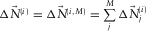 . This update is subsequently summed in terms of i to build the total surface-wave estimate, i.e.,
  , resulting in the surface-wave estimate. Note that the loop is seamlessly closed once the parameters are estimated and the resulting modal surface-wave update
  is obtained. This algorithm can be expressed as
 (6)
(6) (7)
(7) (8)
(8) (9)
(9) (10)
(10)
 ), i.e.,
  , the parameters and/or their updates,
  ,
,  , and
, and  are estimated from the residual update
  . Here,
 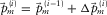 , and
, and  . First, at the parameter estimation/selection module, the dispersion surface
  is estimated by picking the amplitude maxima of the modal surface-wave estimate added to the residual update in the normalized Radon (
 -f) domain. The normalization in the
  –f domain followed by the Radon transform enhances the phase information in the
  –f domain and makes the picks accurate (Park, Miller, and Xia 1998). Equation 4 then provides
  , and the modal surface-wave update
  is subsequently obtained by forward modelling. Second, at the adaptive subtraction module, the source update
  is estimated by solving the global Wiener filter
  obtained by minimizing the following misfit:
 (11)
(11) (12)
(12) (13)
(13) , combined for all frequencies, defines a convolution filter in the time domain. Optionally, the length of this filter in time can be restricted. Third, still in the adaptive subtraction module, the adaptive filter
  is estimated by solving the local (area-by-area) Wiener filter, obtained by minimizing the following misfit:
 (14)
(14) (15)
(15) , combined for all frequencies, defines a convolution filter in the time domain, and the length of this filter in time can be optionally restricted. In practice, for Equation 14, a non-zero diagonal element of
  for a kth receiver location
  can be provided by
 (16)
(16) indicates the trace of a matrix, i.e., the sum of its diagonal elements, in a spatial window centred on the kth receiver location. In Equation 16, the numerator is the cross-correlation of
  and
and  , and the denominator is the auto-correlation of
  . The spatial window of the cross-correlation and the stabilization factor of the auto-correlation control the signal-protecting scheme. A wider spatial window and a larger stabilization factor lead to a Wiener filter protecting the signals
  but probably predicting less energy for the surface waves
  of
of  . A narrower spatial window and a smaller stabilization factor lead to a Wiener filter predicting more energy for the surface waves
  but possibly attacking the signals
  of
of  . This means that there is a tradeoff between conservative signal protection and aggressive surface-wave estimation. The choice of the spatial window and the stabilization factor can be determined by testing.
Figure 2 shows the closed-loop kernel, summarizing the roles of the outer i loop, the inner j loop, the parameter estimation, and the surface-wave updating.

 , the modal surface-wave estimate
  can be obtained for a particular surface-wave mode, i.e.,
  .
.Step-by-step illustration of the closed loop
To illustrate the closed-loop approach, we use 3D ocean-bottom-cable hydrophone data acquired offshore Abu Dhabi in a shallow-water environment. We consider a cross-spread gather consisting of a receiver line in the x-direction and a source line in the y-direction, each with a length of 3,200 m and a spatial sampling interval of 50 m. This represents a 3D cube. Bad traces have been edited. Figure 3 shows the seismic data in the  –t, the wavenumber–frequency (
 –f), and the Radon (
 –f) domain, respectively. Surface waves are clearly seen, distinguishing themselves from subsurface signals by larger amplitudes and lower frequencies. The fundamental mode (
 ) and a higher mode (
 ) can be identified. Each has a cone shape in the
  –t and the
  –f domains, and a hyperboloid shape in the
  –f domain with slowness larger than those of the subsurface signals. In general, a lower mode has larger slowness, producing a narrower cone shape in the
  –t domain, a wider cone shape in the
  –f domain, and a wider hyperboloid shape in the
  –f domain. Aliased energy is observed particularly in the
  -f and the
  -f domains, wrapping around and obliquely intersecting the true energy. Subsurface signals are also found. Refractions lie in a wider cone shape around a smaller two-way time range in the
  –t domain, in a narrower cone shape in the
  –f domain, and in a more cylindrical shape in the
  –f domain, compared with those of surface waves. Reflections appear as flat events, i.e., around tops of hyperboloids, with infinitely small slowness over the whole two-way times in the
  –t domain, and around the origin
  and
and  over the frequencies in the
  –f and
  –f domains.

 –t, (b)
  –f, and (c)
  -f domains, with a vertical section at the top and a horizontal time/frequency slice at the bottom. A dotted line in the section indicates the position of the slice and vice versa. Red, magenta, green, and blue arrows indicate the surface-wave fundamental mode, a surface-wave higher mode, refractions, and reflections, respectively. A filled arrow indicates the true energy, and the whitish versions of the arrows indicate the aliased energy of the various wave types. Notice that the surface waves are dispersive, multi-modal, and aliased.
The initial parameters for the closed loop are either based on a priori knowledge or determined from the seismic data. Figure 4a shows the initial dispersion surfaces  for the fundamental mode and the higher mode. In this example, the initial dispersion surfaces were obtained by manually picking a 1D dispersion curve, e.g., the amplitude maxima of a 2D section in the
  -f domain, and by filling the picks along azimuth at each frequency. Thus, the initial dispersion surfaces have a circular shape in a frequency slice. The initial source wavelets
  were prepared as a spike, minimum-phased and band-limited in the frequency range. The initial adaptive filters
  are zero. Therefore, the initial surface-wave estimate
  is also zero.

For the first loop and the fundamental mode  , the residual update
  (to become also
  ) equals the seismic data
  (see Fig. 3a). Figures 5a and b show the initial dispersion surface
  and the initial source wavelet
  , respectively. First, the dispersion surface
  is estimated. Figures 5c and d show the residual update in the normalized Radon (
 -f) domain, in which
  is estimated by automatically picking the amplitude maxima. As mentioned, the normalization enhances the phase information and improves the accuracy of the picks (see Fig. 3c for comparison). The fundamental mode is clearly seen as a hyperboloid shape with slowness larger than those of the higher mode and subsurface signals. Aliased energy is observed, obliquely intersecting the true energy. To enhance the true energy and make the picks more accurate, optionally, a smoothing filter and a windowing filter along
  can be applied. Figure 5e shows the estimated dispersion surface
  that explains the azimuthal variability (see Fig. 5a for comparison). Figure 5f shows the resulting fundamental-mode update
  . Second, the source update
  is estimated by solving the global Wiener filter
  and multiplying this filter with the initial source wavelet
  . Figure 5g shows the estimated source update
  that explains the source bubble oscillation and ringing (see Fig. 5b for comparison). Figure 5h shows the resulting fundamental-mode update
  . Third, the adaptive filter
  is estimated by solving the local Wiener filter. As mentioned, this filter compensates for model inaccuracies, e.g., related to (intrinsic) attenuation and spatial variability. Figure 5i shows the resulting fundamental-mode update
  . Finally,
  itself becomes the fundamental mode
  at this stage. For the higher mode (
 ), the same procedure is followed. Figure 5j shows the resulting higher mode update
  . Figures 5k and 5l show the total surface waves
  , and the subsurface signals
  after the first loop.
  contains a surface-wave residual at this stage and becomes the residual update
  for the second loop. For subsequent loops, the procedure is iterated until it has reached a stopping criterion. Empirically, we determined that a few iterations are sufficient to converge to a stable solution.

 –f domain without and with a smoothing/windowing filter. (e) and (f) The estimated dispersion surface and the resulting fundamental mode update. (g) and (h) The estimated source update and the resulting fundamental-mode update. (i) The fundamental-mode update after estimating the adaptive filter. (j) The higher-mode update after estimating the adaptive filter. (k) and (l) The estimated surface waves and the resulting subsurface signals after the first loop, with a vertical section at the top and a horizontal time/frequency slice at the bottom. A dotted line in the section indicates the position of the slice and vice versa.
The closed-loop approach estimates the surface-wave parameters (see, e.g., Fig. 4b) and, consequently, estimates most of the surface waves including the aliased energy. However, a residual may still exist in the form of unexplained noise. Optionally, after the closed-loop approach, a conventional slowness/velocity-based filter can be applied to the subsurface signals to further enhance the separation of the subsurface signals from the unexplained noise.
Limitations
At this point, we discuss the limitations of our method. First, as already stated, there is a tradeoff between conservative signal protection and aggressive surface-wave estimation in the adaptive subtraction. The former protects subsurface signals but probably predicts less energy for surface waves, causing a residual of the surface waves in the resulting subsurface signals. The latter predicts more energy for surface waves but possibly attacks subsurface signals, causing a seepage of the subsurface signals into the estimated surface waves. This is also true for surface-wave modes. A part of one mode could leak out into another mode. For example, the fundamental-mode update could contain a part of the higher mode (Fig. 5i), and vice versa (Fig. 5j). This should be controlled by the signal protecting scheme and determined by testing. Second, the method is applied to each basic subset, e.g., each common-source gather. Therefore, the estimated model parameters are representative ones approximated over the spread. An adaptive filter should compensate for the inaccuracies of model parameters and surface-wave estimates in terms of minor variation of phase and amplitude. However, this could not handle sharply discontinuous variation, such as scattering points, within the spread. Third, less energy of surface waves in seismic data makes it difficult to estimate the model parameters and consequently surface waves. However, fortunately, this is not a case in practice. Surface waves are often dominant in seismic data, unless they are somewhat attenuated during the acquisition.
EXAMPLES
We applied our method to 3D ocean-bottom-cable (OBC) hydrophone data in a shallow-water environment and to 3D geophone data in a land environment acquired offshore and onshore Abu Dhabi in order to demonstrate the virtues of the method. Furthermore, we applied our method to irregularly sampled and blended OBC hydrophone data in order to demonstrate its wide range of applicability. In these examples, a conservative signal-protecting scheme was used in the closed-loop approach to avoid distortion of the subsurface signals as much as possible. After that, the closed-loop approach was followed by a conventional slowness/velocity-based filter.
OBC hydrophone data
For the first example, we applied our method to the 3D OBC hydrophone data. We consider a cross-spread gather, consisting of a receiver line in the x-direction and a source line in the y-direction, each with a length of 3,200 m and a spatial sampling interval of 50 m (Fig. 6a). Figures 7a and d show the seismic data  . In fact, these are the same seismic data used earlier in Figures 3–5. Surface waves can be clearly observed, in particular the fundamental mode and one higher mode, both in a cone shape with slowness larger than those of subsurface signals. Severe aliasing is observed, which is well visible in the
  -f domain. Figures 7b, c, e, and f show the estimated surface waves
  and the resulting subsurface signals
  . These results demonstrate that our method successfully estimates the surface waves and separates them out from the seismic data to obtain the subsurface signals. Furthermore, the method estimates even the aliased surface waves for undersampled seismic data.


 –t and
  -f domains with a vertical section at the top and a horizontal time/frequency slice at the bottom. A dotted line in the section indicates the position of the slice and vice versa.
At this point, we compare our method with a conventional slowness/velocity-based filtering method, e.g., in the  –f or
–f or  –f domain. Figure 8 shows the results just after the conventional method. In contrast to the above results with our method, the filtered surface waves do not fully contain the aliased energy. A part of the aliased energy leaks into the resulting subsurface signals. Furthermore, the filtered surface waves contain some unexplained noise in the filtering window. This reveals such a limitation of the conventional method.

 –t and
  –f domains with a vertical section at the top and a horizontal time/frequency slice at the bottom. A dotted line in the section indicates the position of the slice and vice versa.
Irregularly sampled and blended OBC hydrophone data
For the next example, we also applied our method to irregularly sampled and blended seismic data to demonstrate its wide range of applicability. A cross-spread gather, consisting of a spatial sampling aperture of 3,200 m and a spatial sampling interval of 25 m both in the x- and the y-direction, are randomly decimated by 75 %, resulting in an irregularly sampled common-source gather with a spatial sampling interval of 50 m on average in both directions (Fig. 6b). In this case, a conventional slowness/velocity-based filter is not cascaded after the closed-loop approach, since this filter requires regularly sampled seismic data. This would require some regularization step prior to the implementation. Figure 9 shows the results after our method, which estimates the surface waves even for the irregularly sampled seismic data.

 –t domain with a vertical section at the top and a horizontal time slice at the bottom. A dotted line in the section indicates the position of the slice and vice versa.
Furthermore, three cross-spread gathers are synthesized into a blended-source gather consisting of three blended sources and a receiver spread with a width of 3,200 m and a spatial sampling interval of 50 m both in the x-direction and the y-direction (Fig. 6c). The OBC data acquired by stationary receiver spreads are most ideal for synthesizing a blended-source gather. Figure 10 shows the results after our method. Blending of seismic events is well visible. Our method even estimates the blended surface waves without any additional steps for the blended seismic data, such as deblending prior to the implementation. It should be noted that, in this example, the results were obtained from a single blended source gather without using other source gathers simultaneously.

 –t domain with a vertical section at the top and a horizontal time slice at the bottom. A dotted line in the section indicates the position of the slice and vice versa.
Land geophone data
For the last example, we applied our method to the 3D land geophone data. The acquisition geometry is the same as in the first example. The receivers constituted a geophone array. Therefore, surface waves were already somewhat attenuated during the acquisition. The sources configured a Vibroseis array with a linear sweep of 6 Hz–80 Hz. Therefore, with these seismic data, a useful frequency range starts from about 8 Hz in the low frequency side. Figure 11 shows the results after our method. The seismic data are noisy. A considerably large amount of noise, such as coupling noise, scattered noise, etc., which cannot be explained as surface waves, is visible. The surface waves themselves are fully aliased in the whole range of useful frequencies due to their velocity being lower than that in the above examples. Nevertheless, our method reasonably estimates the aliased surface waves even for this noisy seismic data, although some residual exists due to the limitations of the method.

 –t domain with a vertical section at the top and a horizontal time slice at the bottom. A dotted line in the section indicates the position of the slice and vice versa.
CONCLUSIONS AND REMARKS
- It addresses the surface-wave properties such as dispersion and multi-modes.
- It is data driven and data adaptive. This automatically takes into account physical phenomena such as attenuation, anisotropy, spatial variation, etc., which may result from near-surface geological features.
- It can be applied in any geometry domain, such as 3D common shot, 3D common receiver, and 3D cross-spread gathers. Furthermore, it can be applied to undersampled, irregularly sampled, and blended seismic data. This suggests the possibility of relaxing the spatial sampling interval and its regularity, encourages blending and, therefore, offers flexibility with respect to the seismic acquisition geometry.
Finally, it should be remarked that recent advances in seismic acquisition, such as point receivers and a larger amount of stations, make the method more effective because of the improved sampling of surface waves without negative array effects.
ACKNOWLEDGEMENTS
The authors would like to thank Adnoc and their R&D Oil Sub-Committee for their permission to use the data from Abu Dhabi and to publish this paper, Inpex for their financial support for this research, the Delphi consortium sponsors for their support and discussions on this research, and the anonymous reviewers for their constructive comments.