Normal moveout velocity for pure-mode and converted waves in layered orthorhombic medium

INTRODUCTION

In this work, we derive phase-domain azimuthally dependent normal moveout (NMO) velocities for quasi-compressional (qP-qP), quasi-shear (qS1-qS1, qS2-qS2), and converted (qP-qS1, qP-qS2, qS1-qS2) waves in 1D multi-layer orthorhombic media. For simplicity, from now on, we drop the term “quasi” and the prefix “q”, which refer to compressional and shear waves. It is assumed that the vertical orthorhombic axis is the same for all layers, but the elastic properties, the thickness, and the azimuthal orientation of the horizontal orthorhombic axes at each layer may be different. The phase-azimuth-domain moveout approximations are required for analysing azimuthally dependent residual moveout parameters from depth migrated gathers generated in the local angle domain (LAD) by full-azimuth angle domain imaging techniques (e.g., Koren and Ravve 2011 and the references within). The residual moveout curves result from the inaccuracy of the background orthorhombic model parameters used in the migration. For simple to moderate subsurface models, it is common practice to assume laterally varying local 1D models, where, although the model parameters change from location to location, for the residual moveout approximation, it is assumed that, locally, there are no lateral variations. Our derivation is then based on preserving the magnitude and azimuth of the horizontal slowness vector ( and ψ_phs) along the entire ray path in 1D models. It provides the NMO velocity and the NMO as a function of small offsets for each phase azimuth.

Small offset hyperbolic moveout approximations versus surface-offset azimuth for compressional, shear, and converted waves in 1D layered orthorhombic media have been presented by Grechka and Tsvankin (1998, 1999) and Grechka et al. (1999a,b). Thomsen (1999) analyzed the surface-offset-dependent moveout approximations for converted waves in a general inhomogeneous anisotropic medium. Bakulin et al. (2000, 2002) discussed modelling and inversion of the effective parameters for orthorhombic models formed by one or two orthogonal vertical fracture sets embedded in a vertical transverse isotropy (VTI) background, considering reflection moveout of P-P and P-S waves. Parameter estimation in orthorhombic layered media from P-P and P-S data was further explored by Grechka et al. (2005). A detailed discussion about the polarization of the fast and slow shear waves and the computation of their phase and ray velocity surfaces for media with symmetries lower than polar anisotropy has been presented in a recent paper by Grechka (2015). Overall, the offset-domain azimuthally dependent NMO approximations have been intensively explored and used for analysing azimuthal anisotropic parameters, such as intensity and orientation of aligned stress/fracture systems, from time or time-migrated gathers.

It has been shown (e.g., Koren and Ravve, 2011) that full-azimuth imaging in the LAD provides amplitude-preserved angle/azimuth-dependent reflectivity with higher accuracy and higher resolution. Our main aim in this work is to derive the phase-domain NMO velocities to establish explicit approximations for azimuthally dependent second-order residual moveout analysis in this domain, for all types of pure-mode and converted waves. Indeed, for compressional waves in layered orthorhombic media, higher order moveout approximations for longer offsets (wider angles) and for surface-offset azimuths have already been derived (Al-Dajani, Tsvankin, and Toksoz 1998; Grechka and Tsvankin 1998; Pech and Tsvankin 2004), and for phase azimuth by Ravve and Koren (2014) and Koren and Ravve (2015). However, in this work, in addition to compressional waves, we mainly concentrate on shear-wave propagation and converted P-S waves. The use of P-S methods in seismic exploration has been considered in the tutorial by Stewart et al. for isotropic (2002) and anisotropic (2003) media. It has been shown that converted waves experience more severe anisotropy than pure waves (e.g., Cary and Zhang 2010), where the azimuthal anisotropy causes shear-wave splitting of the converted waves into separate P-S1 and P-S2 waves (e.g., Wang, Hollis, and Nowry 2013). We therefore focus on studying the small offset moveout versus phase-velocity azimuth for the different pure-mode and converted waves.

Each layer is characterized by its thickness , azimuthal orientation of its local axis x₁ (local azimuth ), vertical compressional velocity v_P, parameter f (explained in equation (2a) in the following) that depends on the ratio between the vertical shear velocity polarized in x₁ and the vertical compressional velocity, and seven Thomsen-style parameters suggested by Tsvankin (1997); these parameters follow a similar anisotropic discretization for VTI (Thomsen 1986).

In a general anisotropic 1D medium, the horizontal slowness and azimuth of the phase velocity are constant through all layers. This statement follows from Snell's law, and it holds for both pure-mode and converted waves. In our previous study (Koren and Ravve 2014), we derived an analytic relationship for the azimuthal deviation between the phase and ray velocities in each individual layer. This azimuthal lag depends on the local fast and slow NMO velocities and the local “slow azimuth” (azimuth of the slow NMO velocity). With this relationship, we show that the ray-angle- and phase-angle-based approaches yield equivalent effective parameters for a layered azimuthally anisotropic 1D structure. We split the lateral propagation distance (offset) h into two horizontal components: lengthwise , along the phase-velocity azimuth ψ_phs, and transverse , in the normal direction , as shown in the scheme in Fig. 1, where . A right triangle is shown in red, whose legs are and . Leg is in line with the phase-velocity azimuth ψ_phs, and the hypotenuse h is in line with the surface-offset azimuth ψ_off. The acute angle adjacent to leg is .

We establish the local NMO velocities and the lags between the ray and phase-velocity azimuths for individual layers, and we then generalize our findings from pure compressional and shear waves into the three types of converted waves, i.e., P-S1, P-S2, and S1-S2, and from a single layer to multi-layer media. We consider two numerical examples, one with weak anisotropy and the other with strong anisotropic parameters, where the hyperbolic approximations of the travel times are compared with travel times obtained through exact raytracing, studying all types of pure-mode and converted waves, for a multi-layer package. It is clearly seen, especially with strong anisotropy, that the accuracy of the hyperbolic approximations are acceptable only for short offsets, where the ratio between the maximum half-offset to the target depth is not larger than one half (∼27^o half-opening angle). We define the opening angle as the angle between the incidence and reflection slowness vectors, assuming that the two rays emerge from the image point. Note that for compressional waves, the hyperbolic approximation loses its accuracy for strong anellipticities , and for shear waves, the loss of accuracy occurs even for relatively small anellipticity values, in particular for negative anellipticity. However, we show that even with the short offset (small angle) traces of the common image gathers, there is sufficient sensitivity to analyze the azimuthally varying moveout.

The extensive derivations in this study may be found in the Appendices. In Appendix A, we consider the two-way relationship between the surface-offset azimuth (or the ray-velocity azimuth for a single layer) and the phase-velocity azimuth. This relationship is then used to derive the NMO velocity versus phase-velocity azimuth from the well-known formula versus surface-offset azimuth. In Appendix B, we derive the hyperbolic approximations of the lengthwise and transverse offset components and the travel time versus axial values of the NMO velocity ( and ), for both individual layers and the entire multi-layer structure. In Appendix C, we apply these relationships to establish the effective parameters of a layered structure, given the elastic properties of the layers, their thickness and azimuthal orientation, and the wave type. In Appendix D, we demonstrate that the three effective parameters (fast and slow NMO velocities and slow azimuth) can be equivalently calculated in both surface-offset azimuth and phase-velocity azimuth domains. We define S1 as the fast shear wave and S2 as the slow one. are local axes of a given orthorhombic layer, where the three planes of mirror symmetry intersect pairwise, whereas axis x₃ is also the global vertical axis. Vertical shear waves are polarized along the orthorhombic axes x₁ or x₂. When studying the moveout approximations, we consider nearly vertical rays with an infinitesimal horizontal slowness . One nearly vertical shear wave is polarized in the direction close to x₁, notated in this study as Sx₁. For the other shear wave, which is polarized in the direction close to x₂, we use notation Sx₂. The analysis of converted and shear waves in this study is performed on the assumption that the two differently polarized vertical shear wave velocities are different, (or ). For a single orthorhombic layer, should we assume that , then the x₁ polarized wave is S1 (fast), and the x₂ polarized wave is S2 (slow), i.e.,

(1)

Parameters are vertical velocities of the compressional wave, shear wave polarized in x₁, and shear wave polarized in x₂, respectively. We use an auxiliary parameter f, which is related to the ratio between the vertical velocity of x₁-polarized shear Sx₁ and the vertical compressional velocity, i.e.,

(2a)

Thus, the vertical shear velocities can be written as

(2b)

where parameter g shows the ratio between two differently polarized vertical shear velocities, as follows:

(2c)

For rays with an arbitrary direction of propagation, S1 and S2 are shear waves with larger and smaller shear phase velocities, respectively (rather than waves with larger and smaller vertical shear velocities for nearly vertical rays). We emphasize that fast shear means a higher velocity of the wave front propagation (and not necessarily a higher NMO velocity) as compared with the slow shear.

This work deals with a forward calculation of effective NMO velocity parameters for multi-layer orthorhombic models, which can then be used to compute phase-domain azimuthally varying NMO velocity to approximate the moveout. We reemphasize that the proposed moveout approximation in the phase-velocity azimuth domain is particularly important for analysing residual moveouts measured along full-azimuth common image reflection angle gathers. The use of the approximation formulas for the inversion of interval anisotropic velocity parameters is beyond the scope of this paper.

NORMAL MOVEOUT VELOCITY FOR A SINGLE ORTHORHOMBIC LAYER

For a single orthorhombic layer, our relationship for the local normal moveout (NMO) velocity v₂ versus phase-velocity azimuth has the following two generic forms (see Appendix A for derivation):

(3a)

(3b)

where are the local axial NMO velocities in the directions of the local orthorhombic axes x₁ and x₂, respectively, and are the local fast and slow NMO velocities, respectively. These relationships can be compared with the well-known formulas derived by Grechka and Tsvankin (1998), where the local NMO velocity for a single layer is presented versus the ray-velocity azimuth, i.e.,

(3c)

(3d)

where ψ_ray is the ray-velocity azimuth for a given layer. These relationships are valid for any type of pure-mode and converted waves. Equations (3a,c) present the local NMO velocity function versus the local axial NMO velocities related to a given layer. These local axial NMO velocities correspond to the azimuths and , respectively, where is the azimuth of the local orthorhombic axis x₁. The axial NMO velocities are listed in Table 1, where the vertical shear velocities and parameter g are defined in equation (2), whereas σ₁ and σ₂ are

(4)

Table 1. Axial NMO velocities for a single orthorhombic layer

Wave type	Axial NMO velocity	Axial NMO velocity
pure-mode P
pure-mode Sx1
pure-mode Sx2
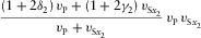
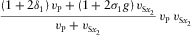
converted
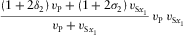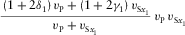converted
converted

Our relationships for the axial NMO velocities for pure-mode compressional and shear waves, summarized in Table 1, match the results first published by Grechka et al. (1999a), which are based on the analysis of the ray-velocity azimuth. Note that, in the orthorhombic axial directions, the azimuths of the ray and phase velocities coincide. It is also important to note that the NMO velocity of shear wave Sx₁ (polarized mainly in x₁) in the azimuthal direction of axis x₂ coincides with the NMO velocity of shear wave Sx₂ (polarized mainly in x₂) in the azimuthal direction of axis x₁, i.e., the constraint holds for any homogeneous orthorhombic layer. Note, however, that this is not true for multi-layer media where the two analogous global effective shear velocities are different, as we will see in a numerical example in the following. Grechka et al. (1999a, 1999b) emphasized that such constraint of shear velocities in the symmetry planes indicates a possible redundancy in the moveout measurements that can be used as a constraint to increase the accuracy of the inversion procedure.

One of the axial velocities proves to be fast and another slow, depending on the relationship between the Thomsen-like parameters. We can establish the local slow azimuth ψ_slow, and we rearrange the local NMO velocity function from equations (3a,c) into equations (3b, d), i.e.,

(5a)

(5b)

The full derivation of the NMO velocity functions for pure-mode and converted waves for a single orthorhombic layer and a multi-layer structure is given in Appendix A. We note that the two-way offset is not equal to the algebraic sum of the one-way offsets (lateral propagations) in the case of converted waves in orthorhombic layered media, due to the varying azimuthal deviations between the phase and ray velocities for the incident and reflected rays. The incident and reflected phase-velocity azimuths are the same due to Snell's law. The incident and reflected ray-velocity azimuths are different in the case of P-S1, P-S2, or S1-S2 converted waves in the orthorhombic medium, as shown in Fig. 2. For a single layer, the lateral propagations of the incident and reflected rays should be added geometrically, i.e., we can add separately the lengthwise components of the lateral propagation along the phase-velocity azimuth ψ_phs, and the transverse components along the normal azimuth . The scheme in Fig. 2 shows a lateral projection of the two-way ray path. The surface offset is shown in the scheme by a red line. Angles and are azimuthal differences between the ray velocity and phase velocity for the incident and reflected waves, respectively. Both azimuthal deviations are known values or known functions of the Thomsen-like parameters and the azimuth of the phase velocity. For converted waves, these angles in the orthorhombic medium are unbalanced, i.e., .

AZIMUTHAL LAG AND NMO VELOCITY FOR A MULTI-LAYER PACKAGE

We distinguish between the local and global azimuthal lags. The local lag is the difference between the ray-velocity azimuth in a given layer and the phase-velocity azimuth. The global lag is the difference between the surface-offset azimuth (acquisition azimuth) and the phase-velocity azimuth. The local lag is related to one-way propagation within a given layer, whereas the global lag is related to two-way propagation along the multi-layer model. The global lag between the surface-offset azimuth ψ_off and the phase-velocity azimuth ψ_phs, as shown in the scheme in Fig. 1, i.e.,

(6)

According to equations (A-1) and (A-2) in Appendix A, the surface-offset azimuth may be expressed through the phase-velocity azimuth and vice versa, i.e.,

(7a)

(7b)

where , and Ψ_slow are the global fast and slow NMO velocities and the azimuth of the global slow NMO velocity, respectively.

The global lag may also be expressed through the fast and slow global NMO velocities, the global slow azimuth, and either phase-velocity azimuth or surface-offset azimuth. It follows from equation (A-5) (written originally for the local lag) that

(7c)

(7d)

Thus, given the three parameters of the global effective model, we can express the global lag either through the phase-velocity azimuth or through the surface-offset azimuth. The global effective NMO velocity versus the phase azimuth and versus the offset azimuth, respectively, reads,

(8a)

(8b)

where equation 8(a) follows from equation (3b), and equation (8b) was suggested by Grechka and Tsvankin (1998). To apply equation (8a) or (8b) for the NMO velocity of a multi-layer structure, we first need to establish the three global effective parameters of that structure: the fast and slow NMO velocities and the azimuth of the slow NMO velocity, i.e., , respectively. With equation (8a) or (8b), we can use the standard hyperbolic moveout approximation

(9)

where h is the surface offset, is the global two-way time, is the global two-way vertical time, and the azimuth ψ may be either the phase-velocity azimuth ψ_phs or the surface-offset azimuth ψ_off. Estimation of the global effective NMO velocity parameters is explained in the following section.

PARAMETERS OF THE EFFECTIVE MODEL

Global effective parameters approximate components of the offset and travel time of a multi-layer orthorhombic model for any azimuth of the phase velocity (or surface-offset azimuth). In this study, the error of the travel-time approximation is , and the errors of the offset components are ; this accuracy is sufficient to establish the three exact global effective parameters for the normal moveout (NMO) velocity. For all types of pure-mode and converted waves, the governing equations for the effective models look alike, but the computed effective parameters are different. According to the formulas in Table 1, we first compute the two axial NMO velocities, and , related to the local orthorhombic axes x₁ and x₂. They depend on the given type of wave. We emphasize that all further equations in this section are generic and may be related to any type of conversion. The full derivation for the global effective parameters is presented in Appendices B and C. After the local axial NMO velocities for the pure-mode waves have been established, we introduce and compute the following local auxiliary parameters () and global auxiliary parameters (),

(10)

The proposed auxiliary parameters have units of velocity squared multiplied by vertical time, and this triad is an analogy of a single parameter for azimuthally isotropic layered medium (e.g., isotropy or vertical transverse isotropy). Parameter is the local azimuth of the orthorhombic axis x₁ for a given layer i. Parameter in equation 10 is the one-way local vertical time for the corresponding type of wave, and all layer auxiliary parameters are summed twice. The local one-way vertical time reads as follows:

(11)

where is the layer thickness, and is the vertical velocity for the given type of wave. Next, we compute the slow azimuth of the global effective model (see Appendix C), i.e.,

(12a)

Finally, the effective fast and slow NMO velocities of a multi-layer package read as follows:

(12b)

where is the total two-way vertical time of the multi-layer package for the given type of pure-mode or converted wave.

DISCUSSION: RESIDUAL MOVEOUT

The main motivation of this study is to provide a tool for residual moveouts (RMO) analysis along phase-azimuth/angle-domain common image gathers, and to provide a mechanism for updating velocity parameters in a layered orthorhombic medium. The RMO analysis and the updating procedure are performed in the depth migrated domain. In this work, we refer to a special imaging technique, where full-azimuth reflection angle domain image gathers are created using a background azimuthally isotropic/anisotropic layered velocity model (Koren and Ravve 2011). Since the background model is normally defined with simpler isotropic and anisotropic characteristics than the true one, RMOs as functions of the opening angles and azimuths can be identified and measured. The residual moveouts can be defined as vertical time errors , and these errors can be associated with the azimuthally dependent variations of the effective NMO velocity . Within the accuracy of the hyperbolic approximation, the travel time is delivered by equation 9. Assuming that the travel time and the offset components are preserved in the background and the updated (true) models, the change in vertical time is the result of the NMO velocity variation, i.e.,

(13)

The sign in equation 13 is assigned so that the variation compensates the RMO . According to equations (B-13) and (7b), the offset approximation versus the phase-velocity azimuth and versus the surface-offset azimuth reads as follows:

(14a)

(14b)

Equations (8), 13, and (14) are valid for any type of pure-mode and converted waves. Combining these equations, we obtain the residual moveout in the phase-velocity azimuth domain and in the surface-offset azimuth domain, i.e.,

(15a)

(15b)

where the effective parameters , the function for the NMO velocity or , and the vertical time are related to the background model. In case of an azimuthally isotropic background effective model (with all layers isotropic or VTI), the relationship simplifies to the following:

(15c)

As a result, we obtain the residual NMO velocity that makes it possible to update the effective fast and slow NMO velocities and the effective slow azimuth, related to the given top and bottom horizons. One can then use a generalized Dix-type inversion (e.g., Koren and Ravve 2014, for compressional waves) to obtain the local fast and slow NMO velocities of the layer and the orientation of its lateral orthorhombic axes. Alternatively, the residual moveout can be used as input for global tomography.

NUMERICAL EXAMPLES

In Fig. 3, the normal moveout (NMO) velocities (divided by the vertical compressional velocity v_P) are plotted versus the phase-velocity azimuth for the pure-mode compressional wave and for the three types of converted waves, with the corresponding shear polarizations, for an orthorhombic medium. The following parameters are used: , , , and . In this example, , and the fast shear wave S1 is polarized as Sx₂, whereas the slow shear wave S2 is polarized as Sx₁. The black line is a pure-mode compressional wave P-P, the red and blue lines are converted waves “compressional to fast shear” and “compressional to slow shear” (P-S1 and P-S2, respectively), and the green line is “shear to shear” converted wave S1-S2. In the phase-azimuth domain, in the case of strong azimuthal anisotropy, the NMO velocity plots may be essentially non-elliptic, as we see, for example for pure compressional wave in Fig. 3.

To evaluate the accuracy of the hyperbolic travel-time approximation versus phase-velocity azimuth , for pure-mode and converted waves, we consider two multi-layer orthorhombic structures, with weak and strong anisotropy. The layer properties for the weak and strong anisotropy structures are listed in Tables 2 and 3, respectively. In Figs. 4 and 5, we compare the travel-time approximation with the exact raytracing solution, and we plot the global lag between the surface-offset azimuth and the phase-velocity azimuth for the weak anisotropy structure. In Figs. 6 and 7, the same analysis is performed for the strong anisotropy structure. The travel time is normalized by the two-way vertical time, and the offset is normalized by the doubled depth of the reflection point, i.e., . In Figs. 4 and 6, we compare the hyperbolic approximation with the travel time obtained as a result of exact numerical raytracing for a package of orthorhombic layers, for all types of pure-mode and converted waves, for weak and strong anisotropy, respectively. In Figs. 4 and 6, the phase-velocity azimuth is kept constant, i.e., (and thus, the global NMO velocity V₂ is also a constant value), whereas the offset h varies. The hyperbolic approximation of the travel time is given in equation 9, where the NMO velocity versus phase azimuth is computed with equation (8a).

Table 2. Weak anisotropy orthorhombic layered structure

Layer	δ1	δ2	δ3	ε1	ε2	γ1	γ2	f
1	0.04	−0.05	0.03	0.05	0.06	−0.03	−0.02	0.72	2.6	0.65	100.8o
2	0.04	−0.06	−0.02	0.04	0.05	−0.04	0.02	0.74	2.8	0.70	50.4o
3	0.03	−0.04	0.05	0.04	0.03	0.05	−0.06	0.75	3.0	1.80	129.6o
4	0.03	−0.05	0.04	0.07	0.06	0.06	−0.04	0.76	3.5	1.40	63.0o
5	0.06	−0.05	0.03	0.05	0.02	0.04	−0.07	0.78	3.8	1.90	117.0o

Table 3. Strong anisotropy orthorhombic layered structure

Layer	δ1	δ2	δ3	ε1	ε2	γ1	γ2	f
1	0.05	−0.12	0.03	0.15	0.08	−0.03	−0.02	0.72	2.0	0.65	100.8o
2	0.15	−0.08	−0.02	0.20	0.12	−0.04	0.02	0.74	2.8	0.70	50.4o
3	0.12	−0.06	0.05	0.25	0.09	0.05	−0.06	0.75	3.5	1.80	129.6o
4	0.20	−0.10	0.04	0.30	0.10	0.06	−0.04	0.76	4.5	1.40	63.0o
5	0.17	−0.08	0.03	0.23	0.14	0.04	−0.07	0.78	3.8	1.90	117.0o

To establish the exact numerical value of the travel time, for each value of the opening angle we compute the two-way travel time and the offset between the source and receiver. For this, we first obtain the incidence and reflection angles separately, applying Snell's law at the reflection point, and we then trace each of the two rays independently. For the lowermost layer, the direction of the phase velocity is known, and applying the Christoffel matrix, we can find the absolute value of the phase velocity (taking the root of the cubic equation corresponding to a given type of wave) and therefore the slowness components. For all other layers, lateral slowness components are kept constant, whereas the vertical slowness component p₃ is obtained from the Christoffel equation. We assume that the smallest vertical slowness corresponds to the compressional wave, whereas two others correspond to shear waves (medium vertical slowness to S1 and large to S2). We then check our assumption, computing the three phase velocities v_phs for fixed directions, in order to pick the proper root for p₃. Thus, we know the magnitude and direction of the phase velocity for all layers. Next, we find the polarization, the ray velocity components, the two components of the offset, and the travel time (Vlaar 1968; Červený et al. 1977; Červený 2001). As we see, the hyperbolic approximation is accurate for small offsets and sometimes for moderate offsets. As expected, for the strong anisotropy structure, the error of the hyperbolic approximation grows much faster with the offset increase. In Tables 4 and 5, we present the effective models for the given multi-layer packages, considering all six types of pure-mode and converted waves. Recall that the fast shear S1 has a higher phase velocity (in this case – a higher vertical velocity and shorter vertical time) than the slow shear S2, but the NMO velocities of S1 are not necessarily higher than those of S2. In Figs. 5(a,b) and 7(a,b), we present the absolute error between the exact numerical result and the hyperbolic approximation of the normalized travel time versus normalized offset, for weak and strong anisotropy and for pure-mode and converted waves, respectively, for the fixed phase-velocity azimuth . The absolute error E of the normalized travel time is shown in the graphs, where the normalizing factor is the vertical time, which means that the two-way reflection travel time error is , where is the two-way vertical time. The error graphs in Fig. 5(a) are related to travel-time approximations in Fig. 4(a–c) (weak anisotropy, pure-mode waves), the error graphs in Fig. 5(b) are related to the approximations in Fig. 4(d–f) (weak anisotropy, converted waves), the error graphs in Fig. 7(a) are related to the approximations in Fig. 6(a–c) (strong anisotropy, pure-mode waves), and the error graphs in Fig. 7(b) are related to the approximations in Fig. 6(d–f) (strong anisotropy, converted waves).

Table 4. Effective models for the weak anisotropy layered structure

Wave type			Ψslow
P-P	3.327	3.157	105.31o	4.000
S1-S1	1.805	1.758	138.23o	7.455
S2-S2	1.918	1.742	12.64o	8.162
P-S1	2.441	2.349	111.90o	5.727
P-S2	2.398	2.381	0.18o	6.081
S1-S2	1.852	1.763	5.74o	7.809

Table 5. Effective models for the strong anisotropy layered structure

Wave type			Ψslow
P-P	3.807	3.404	97.17o	3.801
S1-S1	2.301	1.993	121.15o	7.103
S2-S2	2.505	2.023	18.25o	7.743
P-S1	2.902	2.590	108.14o	5.452
P-S2	2.846	2.726	34.59o	5.772
S1-S2	2.286	2.146	5.07o	7.423

In Figs. 5(c,d) and 7(c,d), we plot the corresponding graphs for the global lag between the surface-offset azimuth and the phase-velocity azimuth, versus the normalized offset. In these plots, the phase-velocity azimuth is kept constant, i.e., . These graphs are plotted by numerical raytracing because the hyperbolic approximation can predict this lag only for an infinitesimal offset and does not provide the dependence of this lag on the offset (note that a fourth-order moveout approximation is required to obtain second-order approximation of the azimuth lag). The graphs show that the global azimuthal lags may be essential. In these examples, for the chosen phase-velocity azimuth, the lags may reach 3.5^o for weak anisotropy and 6^o for strong anisotropy structures. The local azimuthal lags between the ray and phase velocity directions may be even greater, as the lags in different layers often compensate each other partially. The global lags vary in a wide range with the offset and may even change the sign, i.e., the surface-offset azimuth may actually lead or lag behind the phase-velocity azimuth. For very long offsets, the global lag converges to its asymptotic value, which is equal to the local lag between the ray and phase velocities of the layer with the fastest phase velocity in the horizontal symmetry plane, for the given azimuth.

Figs. 5(e,f) and 7(e,f) show the effective fast and slow NMO velocities and effective slow azimuths for all types of waves and for weak and strong anisotropy models. As we see, for a multi-layer structure, the orientation of the effective slow azimuth Ψ_slow depends on the specific type of pure-mode or converted wave. Thus, for six wave types, we obtain six different values. This is not so for a single orthorhombic layer, where the slow azimuth coincides with one of the local axes .

In Figs. 8 and 9, the normalized offset is kept fixed, i.e., , whereas the azimuth of the phase velocity runs all values. Equation 9 is used to approximate the travel time, where is now a varying function of the phase azimuth. Blue and red solid lines are approximations for weak and strong anisotropy, respectively. Blue and red dashed lines are the corresponding exact solutions. Label “Ex” means an exact numerical raytracing solution, and label “Ap” means the hyperbolic approximation. In Fig. 8, we compare the hyperbolic travel-time approximation with the exact solution, for all types of waves. In Fig. 9, we plot the lag (between the surface-offset azimuth and the phase-velocity azimuth) versus phase-velocity azimuth, for all types of waves. Within the entire range of the phase-velocity azimuth, the maximum global lag reaches 15^o (Fig. 9c, strong anisotropy, pure-mode wave S2-S2, ). Note that in the case of strong anisotropy and pure-mode shear waves, the exact values of the travel time (versus phase-velocity azimuth) may be unsmooth (Fig. 8b), and the azimuthal lag may even be discontinuous (Fig. 9b), due to shear-wave cusps or close-to-cusp conditions. These points are candidates for the shear-wave singularities extensively studied by Crampin (1981, 1991), Brown, Crampin, and Gallant (1992), and Vavryčuk (1999).

The hyperbolic approximation is always smooth and continuous. However, even in these cases, the smooth continuous prediction of the travel time gives a reasonable quantitative insight (for short offsets), indicating the locations and values of minima and maxima, and the average rates.

CONCLUSIONS

We have derived the normal moveout (NMO) velocity formula for quasi-compressional, quasi-shear, and converted waves, considering two types of shear polarization, for a 1D package of orthorhombic layers versus their common phase-velocity azimuth. This phase-azimuth-domain NMO velocity is required for analysing residual moveouts along local-angle-domain (LAD) common image gathers. The azimuthally dependent NMO velocity formula consists of three independent global effective model parameters (fast and slow NMO velocities and the azimuth of the slow NMO velocity), defining a single layer that yields the same azimuthally dependent moveout as the whole package of layers. Note that the global effective “layer” is generic and not necessarily orthorhombic. To model the global effective NMO velocity for pure-mode and converted waves, we need the given azimuthal orientation of the orthorhombic axis x₁, the vertical compression velocity v_P, the shear-to-compression ratio f (where shear is Sx₁), and all Thomsen-like parameters of the orthorhombic medium, except δ₃, which has no effect within the hyperbolic approximation. It has been demonstrated that when the ratio between the half-offset to the target depth is less than one half (about 25° half-opening angles), the comparison of the azimuthally dependent hyperbolic approximation of the moveout with the exact raytracing-based travel time still demonstrates satisfactory accuracy, even for strong anisotropy and converted waves.

LIST OF SYMBOLS