

Agri-environmental Policy and Urban Development Patterns: A General Equilibrium Analysis
The authors are grateful to two anonymous referees and the editor for helpful comments and suggestions, and also thank Pierre Dupraz and Guy Garrod for their valuable comments on earlier drafts. Financial support from the French Ministry of Environment (PAYTAL - convention 11-MUTS-PDD-3-CVS-019), the Region Pays de la Loire, and the European Union under the Marie Curie Intra-European program (FP7-PEOPLE-2010-IEF - 273191 - LUPUS) are gratefully acknowledged.
Abstract
This paper investigates the spatial effects that the provision of environmental public goods have on residential location choices in a suburban context. Specifically, a spatial general equilibrium framework is developed to analyze the consequences of adopting an agri-environmental policy promoting the provision of positive farming externalities. We use a static monocentric model of an open city where agricultural bid-rents and agricultural amenities vary endogenously in space, and where the positive externalities associated with agricultural production are valued by households. Consistent with empirical evidence of the potential side effects that conservation policies may have in terms of urbanization patterns and land price changes, we show that under certain conditions implementing an agri-environmental policy may promote additional suburban development. Moreover, we demonstrate that the emergence of disconnected suburban areas may be significantly influenced by the location of land regulated by an agri-environmental policy. Finally, we discuss distributional aspects and show that while introducing an agri-environmental policy has a negative impact on most residential land value, it can have positive effects on farmland and residential land located within the regulated areas, suggesting the non-neutrality of such policies regarding the agents' assets.
Agri-environmental programs (AEPs) are policy instruments designed to deliver environmental services by paying farmers to reduce the negative externalities of agricultural production and, in some cases, to deliver positive externalities through environmental management. Baylis et al. (2008), Claassen, Cattaneo, and Johansson (2008), and Wunder, Engel, and Pagiola (2008) conducted in-depth reviews of AEPs in various countries. However, due to the spatial heterogeneity of farming externalities, AEPs cannot be expected to be spatially neutral and have no effect on development patterns, particularly in nearby urban and peri-urban areas (Lewis, Barham, and Zimmerer 2008). Even so, it is acknowledged that the positive externalities associated with farming are valued by residents and that maintaining traditional agricultural landscapes can increase the prices of adjacent properties (Bastian et al. 2002; Anderson and West 2006; Bergstrom and Ready 2009; Klaiber and Phaneuf 2010). Thus, it is reasonable to assume that implementing AEPs can have side effects and may have a local impact on development, especially when they operate close to urban areas.
Both land-use (Quigley and Rosenthal 2005) and environmental regulations (Kiel 2005) have been shown to have the potential to generate important spillovers. For example, Quigley and Swoboda (2007) have shown that programs such as the Endangered Species Act, which can lead to land designation, have impacts that extend beyond the protected areas. Because designated areas are generally exempt from development, urban rents tend to increase in adjacent areas, thereby modifying development patterns and leading to significant redistributive impacts among residents and landowners.
Empirical investigation into the impacts of AEPs on urban development are rare. In the United States, some studies support the idea that AEPs can induce suburban development. Roe, Irwin, and Morrow-Jones (2004) find that the amenity value of preserved agricultural landscapes can be high enough to offset the additional transportation costs associated with this lifestyle, and can thus encourage development at a certain distance from cities. Irwin and Bockstael (2004) have shown that policies aimed at preserving open spaces may induce development on neighboring land. Similarly, Towe (2010) finds that areas of land managed under the Conservation Reserve Program (CRP) in the United States have significant effects on surrounding land, doubling their probability of development and thus modifying development patterns. In Europe, where land preservation is often concealed within urban zoning policies, Geniaux and Napoléone (2011) find that agricultural designation areas in France have significant effects on development patterns.1
Despite their importance, working land programs received little attention with respect to their impacts on urban development patterns.2 The purpose of this article is to examine, from a theoretical standpoint, the potential side effects that AEPs have on urban development, as well as the associated redistributive effects among landowners. To accomplish this, we construct a static monocentric model of an open city, where both agricultural bid-rents and farming amenities vary endogenously in space. In addition, the positive externalities associated with agricultural production are valued by households.
Previous work on the link between amenities and urban sprawl patterns by Wu and Plantinga (2003), Wu (2006), and Kovacs and Larson (2007) relies on exogenous amenities. We depart from the approach used in these studies by making farming amenities endogenous to our model. As in Cavailhès et al. (2004) and Bento, Franco, and Kaffine (2011), amenities are considered endogenous because they depend on the total amount of land in agriculture outside the city that is affected by urban development. We add a new dimension by specifying that the level of farming externalities depends on farming intensity, which is in turn related to the cost of land. Close to cities, farmland is expensive and is substituted by non-land inputs (Beckmann 1972). Moreover, we introduce a voluntary agri-environmental policy, funded by households through a local lump-sum tax, that is aimed at limiting farming intensity. Whether or not farmers adopt the AEP depends on their level of intensification and is thus spatially heterogeneous, which is in line with empirical findings on the adoption of AEPs (Lynch and Lovell 2003). We make some restrictive assumptions to keep our model as simple as possible, and focus on the effect that the AEP has on urban patterns and land rents. Our model is static and thus describes long-run equilibrium development patterns.
The remainder of this article is organized as follows. We first present the model, discuss the adoption of the AEP by farmers, and describe the conditions for a spatial general equilibrium. We then present a numerical illustration with plausible parameters, and finally explore the impact that AEPs have on urban structure and land values.
A Theoretical Model for Location Decision with Endogenous Amenities
This section describes our spatial model and its equilibrium. Since our spatial configuration is circular and symmetric, we place ourselves on a transect with the central business district (CBD) located at its origin, 0. The distance between the CBD and any point on the real line  is x. All non-agricultural employment is concentrated in the CBD. Land is either dedicated to agricultural or residential use in accordance with the rents offered by these two activities. We assume that all land is owned by absentee landlords.
Farmers' Behavior
 . The demand function of non-land inputs is found by maximizing profit π(k,x) with respect to k:
 (1)
(1) (2)
(2)From equation (2),  , meaning that
  decreases with distance to the CBD, and
  tends toward
  where farming is no longer influenced by the city. The limit of the urban-influenced area
  solves
  . Without a loss of generality, we set
  exogenously.
Under our approach, the negative farmers' bid-rent gradient is due to the imposed Thünenian behavior, as in other similar studies introducing farmers' behavior into a monocentric city model (Cavailhès et al. 2004; Caruso et al. 2007). In other words, farming at the urban fringe is intensive in terms of non-land inputs such as labor, capital, equipment, or fertilizers. Further away from the city, agriculture relies more on land. This Thünenian spatial organization has been thoroughly described in the literature (Beckmann 1972; Katzman 1974; OECD 2009) and continues to be a valid explanation of the spatial organization of contemporary suburban agriculture in U.S. and European cities (Heimlich and Barnard 1992; Plantinga, Lubowski, and Stavins 2002; Cavailhès and Wavresky 2003; Livanis et al. 2006; Cavailhès and Wavresky 2007; Wu and Lin 2010). This organizational structure can be related to the location of storage and agri-food facilities at city boundaries, and to the fact that farmers engage in direct sales strategies aimed at local urban populations. However, as highlighted in these studies, there is another important reason that explains the progressive decline of farmland prices as one moves away from the city. This reflects the capitalization of a growth premium, corresponding to expected rent increases based on the potential for the conversion of land to residential use (Capozza and Helsley 1989). Introducing a growth premium would involve a time-dependent process, which cannot be accommodated in our static approach. However, our model is fully compatible with this reality and should be interpreted in this way.
Agri-environmental Policy
We introduce a stylized version of an AEP designed for working land. Our AEP consists of a voluntary contract between the city government and farmers, and aims to reduce the use of non-land inputs, k, to a fixed target,  . In return, all participating farmers are granted a uniform subsidy, σ, per hectare. Farmers decide whether or not to enter into a contract based on their private opportunity costs.4 The proposed AEP is thus fully described by
  . This AEP mimics the voluntary working land conservation programs described in Wunder, Engel, and Pagiola (2008) and Baylis et al. (2008). In many cases, AEPs may be non-uniform, accounting for geographical and environmental heterogeneity across space. We choose not to consider these more complex spatially targeted policies, and instead focus on a simplified general case where a uniform policy is applied across all eligible land.
Farmers' participation in the AEP is endogenous to the model and depends on their location, which in our case fully describes their opportunity cost. Farmers' participation in AEPs has been well documented in the literature and has been shown to depend on factors relating to contract design5 and farmers' characteristics.6 Surprisingly, reviews of participation in AEPs by Knowler and Bradshaw (2007) and Baumgart-Getz, Prokopy, and Floress (2012) suggest that most of these factors are incomplete descriptors of farmers' adoption of these schemes. Still, these two reviews did not identify studies where proximity to urban areas is a determining factor in farmers' participation in AEPs.7 Indeed, such studies are rare but tend to agree that the probability of participating in agricultural land preservation programs is lower close to the city but increases for those farmers located further away from the city (Lynch and Lovell 2003; Van Huylenbroeck et al. 2005; Bertoni et al. 2011).
 (3)
(3) are not granted any subsidy, although it would be interesting for them to adopt the contract since they already comply with the input restrictions (see figure 1). This critical distance is given by
  , from which we derive:
 (4)
(4)
Definition of the contracted area
 do not adopt the measure, as the subsidy fails to compensate them for the loss of profit. Thus,
  solves as:
 (5)
(5) and
and  agree to adopt the measure, and are granted the subsidy (see figure 1). The spatial distribution of farming intensity is then given by:
 (6)
(6)As depicted in figure 1, choosing  is equivalent to choosing the adoption distance
  , and choosing σ is equivalent to choosing the depth
  of the regulated area.
 (7)
(7)Joint Production of Agricultural Externalities
 (8)
(8)Intensive farm systems tend to generate less attractive landscapes and environmental systems of lower quality than more extensive farming (Abler 2001; Maier and Shobayashi 2001; Bergstrom and Ready 2009). However, the relationship between agricultural activity and the provision of rural externalities may be complex, as discussed by Hodge (2000), Harvey (2003), and Wossink and Swinton (2007). This relationship can be competitive: an increase in the level of inputs leads to a decrease in environmental quality, as reflected in cases such as the United States or Australia. In the European case, the relationship between the level of agricultural outputs and rural services may not be monotonous. By specifying the production function of rural externalities in equation (8), we choose to consider a competitive relationship only, which is closer to the U.S. case. In our model, the introduction of an agri-environmental policy regulating the use of non-land inputs will therefore have a direct effect on the provision of agricultural externalities, which was empirically confirmed by studies carried out, for example, by Glebe (2007) or Duke et al. (2012). The regulated area will therefore be characterized by a higher net flow of externalities.
Additionally, the introduction of δ allows us to assume that some types of farming are more inclined to provide amenities than others at any given level of non-land input intensity. The variable δ describes the degree of jointness between amenities and farming. In our model, agriculture such as single-crop farming or soil-less livestock breeding are supposed to generate only a low level of amenities that are positively valued by households (low δ). On the other hand, grasslands or fruit horticulture is supposed to provide a higher level of such amenities, regardless of the use of non-land inputs (higher δ). The value of δ is likely to vary between cities and countries depending on the prevalent farming types and cultural characteristics. For example, in Kentucky horse farms with stone and plank fences, picturesque barns, and grasslands are likely to be associated with a high δ, as described by Ready, Berger, and Blomquist (1997). In Wyoming (Bastian et al. 2002), this would be the case for areas dominated by elk habitat and scenic grasslands. Fausold and Lilieholm (1999), McConnell and Walls (2005), and Bergstrom and Ready (2009) provide insightful reviews of the values associated with farmland and farming.
The variable δ is fixed because our model only relies on one type of farming. Our model could also accommodate several agricultural outputs, with different δ's. Depending on their specific bid-rents, all types of farming would continuously appear spatially one after the other, as shown by Beckmann (1972). However, the uneven spatial distribution of climate, soil, and agronomic conditions, as well as the existence of agglomeration externalities, favor some degree of farming homogeneity and specialization at the city level. Furthermore, introducing different types of farming would add unnecessary complexity to the model.
Households' Location Decisions in Urban and Suburban Areas
Household utility function is determined by the usual trade-off between accessibility to the CBD, land consumption, and amenities. Each household chooses a combination of residential space, qh, location, x, and a numeraire non-housing good, s, to maximize its utility, subject to the budget constraint w=r(x)qh+s+τx+η, where w is the gross household income, τ is the round-trip commuting cost per unit of distance, r(x) is the housing price at location x, and η is a lump-sum tax applied to all households, which is designed to fund the AEP.
We retain a Cobb-Douglas utility function 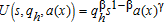 , where a(x) represents amenities. Inside the city, a(x) represents urban amenities only and is equal to unity (a(x)=1). Outside of the city, a(x) corresponds to farming amenities and spatially varies as described in the next section. We suppose that there are no spillovers and that amenities are consumed by households only within their residential location. This assumption is valid as long as we consider localized externalities, such as particular landscape features, open spaces, hedgerows, trees, or visual and olfactory nuisances. The empirical literature shows that the value of open space amenities rapidly decays with distance (Irwin and Bockstael 2004; Cavailhès et al. 2009) to become insignificant beyond a few hundred meters. On the other hand, diffuse amenities such as biodiversity, or disamenities such as water pollution or erosion, may have a much wider spatial impact and are therefore not the types of amenities treated here.
 (9)
(9) (10)
(10) (11)
(11) (12)
(12)These bid-rent functions describe households' maximum willingness-to-pay for housing at location x. In equilibrium, households are indifferent about where they locate because their equilibrium level of utility is the same at each location, and exogenous from the perspective of a single open city. From (11), we observe that the urban bid-rent decreases with distance and equals zero at x=(w−η)/τ. The peri-urban bid-rent (12) distribution across space is more difficult to predict. It is not necessarily a strictly decreasing function of distance, as households may outbid farmers in remote locations where, although commuting costs are high, they can enjoy higher levels of amenities. This bid-rent is similar to that found elsewhere in monocentric models dealing with amenities (Brueckner, Thisse, and Zenou 1999; Wu and Plantinga 2003; Wu 2006).
Farming Amenities
 (13)
(13)Spatial Equilibrium
After deriving farmer and household behavioral functions, we now characterize spatial equilibrium within the urban area. Housing prices are pushed upwards in desirable locations, so that in equilibrium no household wants to move. This condition is satisfied when housing prices are given by equations (11) and (12) and farmland rent is given by equation (7). Land is occupied by the highest bidder. The prevailing land rent at any location is given by 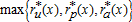 .
.
Definition of the City
 , which is the distance at which agriculture becomes exogenous. The city boundary
  solves
  .9 The city is represented by the set of locations
 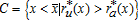 ;
;  is thus determined by the competition between urban households and farmers for land. The number of households
  at any location within the city is defined by:
 (14)
(14) is the residential plot size (in m2/households) and D(x) is the quantity of housing per unit of land (residential plot size per hectare in m2/ha). For simplicity, we suppose that D(x) is given exogenously. This assumption allows us to avoid the introduction of a developer, as is the case in several other models (e.g., Wu 2006; Quigley and Swoboda 2007; Bento, Franco, and Kaffine 2011). This assumption comes at no cost with respect to the interpretation of the model. However, it does preclude us from deriving changes in the housing density.
Definition of the Peri-urban Area
Within the peri-urban area, land is shared between farmers and households. The mixed land-use, peri-urban area is defined by the set of locations  .
.
Two possible configurations arise:
Urban extension: The peri-urban area develops directly from the city boundary  . In this case, x2 must exist such that for all
  , we have
  . Beyond x2, the land is exclusively in agricultural use
  .
.
Leapfrog development: Within our context, we define leapfrog as a pattern of land development that is disconnected from the city. The variable P is not connected to C if  exists, such that for
  we have
  , that is, agricultural use only, and for x∈[x1,x2], we have
  .
.
Characteristics of the Peri-urban Area
 (15)
(15) are, respectively, the number of farmers and households at x within the peri-urban area, and L(x) and
  represent their respective space consumption. Constant returns to scale do not allow us to determine
  and L*(x) separately. Thus, the total number of farmers
  is indeterminate. However, this is not a problem for characterizing the model equilibrium, as we do not focus on landowners and density distributions. All agricultural land could either be run by one single farmer, or by a multitude of small farmers, and land use patterns remain unchanged. As
  and
and  in the mixed land-use area, we derive the level of amenities within the peri-urban area in equilibrium:
 (16)
(16) (17)
(17)Population in Equilibrium
 (18)
(18)Budget in Equilibrium
 (19)
(19) (in ha).
Spatial General Equilibrium
The spatial general equilibrium can be simplified into the 8-uple  defined by equations (11), (17), (18), and (19), the boundaries being defined in the text.
Comparative Static Analysis
The complete comparative static analysis of the model was performed without an AEP.10 The results are consistent with the usual effects highlighted by classic monocentric city models: higher income and lower commuting costs lead to an increase in urban and peri-urban development. The assumption of agricultural heterogeneity across space makes variations of agricultural parameters non-neutral with regard to the peri-urban bid-rent, and therefore to the size and location of the mixed land-use area. When prices of agricultural inputs and outputs vary, the peri-urban households' residential tradeoffs may be affected by the change in agricultural intensity, and therefore amenity provision. However, in our model, introducing the AEP implies a segmented space where various configurations may occur in terms of the relative locations of the regulated and the mixed land-use areas. This leads to more complex non-linear relationships and contradictory effects that cannot be solved analytically. The main economic mechanisms involved when the AEP is introduced into the model are the following. Since the policy is funded by a tax on individual households, a larger regulated area leads to a higher tax income. From equation (11) we have ∂ru/∂η<0, meaning that urban households are negatively affected by the introduction of the AEP. It follows that the impact on urban variables, such as location of the city boundary and total urban population, is similar. However, the effects on peri-urban households are more difficult to predict. The negative effect of taxation may be counterbalanced by an increase in the supply of local environmental amenities arising from the AEP, which has a positive impact on the peri-urban bid-rent (from equation (12) we have ∂rp/∂a(x)>0). The global effect depends on the location of the regulated area, which also determines the effects on Θ*(x) and Np. The comparative static analysis on agricultural parameters regarding the parameters of the AEP is more simple to determine. From equations (4), (5), (6), and (7), we obtain the results in table 1.
 on Agricultural Variables
 |
k* |  |
 |
||
|---|---|---|---|---|---|
| σ |  |
+ 0 | 0 | 0 | – |
 |
 |
+ 0 | + 0 | – | – |
Given the complexity of the model, we choose to visualize the various effects of the AEP through numerical simulations.
Numerical Model
Following Wu and Plantinga (2003), Bento, Franco, and Kaffine (2006), and Wu (2006), we run a set of numerical simulations to visualize the equilibrium patterns of the model and to establish both the direct and indirect effects of the model parameters.
The model's structural parameters are set to simulate a plausible medium-sized French city, using data from the French National Institute of Statistics and Economic Studies (INSEE)11 and the Farm Accountancy Data Network (FADN).12 Parameter values are presented in table 2. According to the income survey conducted by INSEE, between 2000 and 2009 the average income for French households was €33,384, and approximately one-quarter of their total expenditures was devoted to housing (25.6% in 2010). Commuting costs for households are calculated by the French Internal Revenue Service to be roughly €0.40/km. Assuming there are 1.5 workers per household travelling to and from the CBD throughout the year, we set τ=400 €/km/year. Finally, in order to generate a realistic urban bid-rent at the CBD, we set the equilibrium utility value to  . Given the lack of relevant data on household preferences for the amenities associated with AEPs, we arbitrarily set γ=0.2.
| Parameter | Value |
|---|---|
| w Income level | 33 000 € |
| τ Commuting cost | 400 €/km/year |
| β Housing budget share | 0.25 |
 Equilibrium utility level Equilibrium utility level |
10, 100 |
| γ Preference for amenities | 0.2 |
| p Price of agricultural output | 2.62 €/output unit |
| p k Price of non-land input | 1 €/input unit |
| α Elasticity of production factor | 0.8 |
| t Transport costs for farmers | 0.02 €/km/output unit/year |
| A Technical constant | 1 |
| δ Farming-amenity degree of jointness | |
| Urban extension case | 24 |
| Leapfrog case | 18 |
The proportion of non-land costs per hectare reported in the FADN is approximately 90% of the total cost, and provides an average level of charges pkk*=1,861 €/ha per farm, and an average gross product of pAk*α=1,714 €/ha per farm in 2009. Combining this with the estimated proportion of non-land costs per hectare, we obtain a ratio between the output price and the non-land input price of €2.85. We assume that this ratio is constant for an average French farm. We set α=0.8, pk=1 and p=2.62 in order to generate realistic values. Transportation costs for farmers are set to t=0.02 €/km/output unit, so that the radius of the total available land under the influence of the urban area is  .
.
Development patterns are depicted in figure 2. We show two possible sprawl patterns: urban extension and leapfrog development. The occurrence of these scenarios depends, to some extent, on the capacity of agriculture to provide amenities, (δ). Figure 2a illustrates a case where the mixed land-use area is disconnected from the city. We define this urbanization pattern as leapfrog development, which occurs when δ is relatively low (i.e., δ=18). The mixed land-use area is disconnected from the city when the surrounding agricultural activity has a low capacity to provide amenities. The second benchmark configuration depicted in figure 2b is characterized by a peri-urban area located adjacent to the urban area. This urban extension development pattern occurs when farming has a higher degree of joint-production of amenities.

Benchmark patterns of development, leapfrog and urban extension
The main characteristics of both benchmark cities are summarized in table 3. The size of the mixed land-use area and the number of peri-urban households are higher in the case of urban extension. This is due to household preferences for amenities (γ) remaining equal in both cases. An increase in the capacity of agriculture to provide amenities strongly encourages households to move in.
| Description | Variable | Benchmark | |
|---|---|---|---|
| Urban extension | Leapfrog development | ||
| δ | Capacity for a farm to provide amenities | 24 | 18 |
 |
Radius of the city (km) | 13.61 | 13.61 |
| (x2−x1) | Size of the periurban area (km) | 47.67 | 30.17 |
| N u | Number of urban households | 240,505 | 240,505 |
| N p | Number of peri-urban households | 254,527 | 66,944 |
 |
Mean fraction of agricultural land within the peri-urban area (%) | 0.88 | 0.73 |
Effects of Agri-environmental Policy
Farms that are close to the city tend to be intensive and farmers may not be interested in reducing their non-land inputs unless they receive substantial compensation. Therefore, an agri-environmental policy can be designed to encompass land that is either closer to or more distant from the city's boundaries. This decision depends on the level of payments made to farmers (σ) and the restrictions placed on non-land inputs  . Thus, there is a significant potential for agri-environmental policy to be involved in spatial organization within nearby cities and to participate in the shaping of the suburban area.
Impact on the Urban Structure
This section examines the effects of AEPs on the urban structure through some key description variables, that is, location of the urban boundary and size of the peri-urban area.
Urban boundary
The effects of the AEPs on the size of the urban area are depicted in figures 3a and 3b for the urban extension and leapfrog cases, respectively. As urban households do not value agricultural amenities, their bid-rent function remains unaffected by a change in the supply of amenities. However, as urban households are taxed in order to fund the program, an increase in the level of subsidy leads to a decrease in their urban bid-rent  . Consequently, as the participating area increases in size (i.e., low
  and high σ), the location of the urban boundary tends to come closer to the CBD, which is indeed what we observe in figures 3.a and 3.b for approximately σ>100 €/ha and
  non-land input units. In addition, farmers who agree to participate in the AEP capitalize the subsidy in their bid-rent function so that it increases. In cases where participating farmers are located at the urban fringe (i.e., high
  and high σ), farmers can outbid urban households. This explains the negative impact observed for σ, which varies from 200 to 300 €/ha, coupled with
  non-land input units.

Effect of the AEP on  in km
in km
From this simulation, it appears that an ambitious agri-environmental policy, funded by all inhabitants, could theoretically reduce the size of the city. In practice, this may be a real hindrance to urban development in both benchmark scenarios. Obviously this result depends on the assumption of an open city that allows both costless in- and out- migration, but it still shows the non-spatial neutrality of a public policy that supports the provision of a public good such as agricultural amenities.
Size of the Peri-urban Area and Development Pattern
The effect of AEPs on the size of the peri-urban area is more complicated. Figures 4a and 4b depict the variation in the size of the peri-urban area (x2−x1) induced by various combinations of  , compared to the benchmark cases. We consider these variations in the leapfrog and urban extension configurations, respectively. We observe two main antagonist effects following the introduction of AEPs. The first effect is the reduction in the size of the mixed land-use area as a result of peri-urban households being taxed to fund the policy. The decrease in the peri-urban bid-rent, combined with an increase in the agricultural bid-rent following the capitalization of the subsidy, leads to a situation where farmers can outbid households. As a consequence, the peri-urban area tends to become smaller. However, the increased supply of local environmental amenities generated by the policy is an incentive for peri-urban households to move into the area
  . Depending on the location and magnitude of the area under the AEP, the negative impact of the additional taxation required to fund the scheme can be compensated with the increased amenity level provided by those farmers who participate in it. Farmers located in the adoption area can therefore be outbid for land by peri-urban households, thus leading to a larger peri-urban area.

Effect of the AEP on (x2−x1), by percentage
In the leapfrog case (figure 4b), the negative tax effect is clearly visible at high levels of subsidy (σ>150 €/ha) and intermediate and low levels of maximum non-land inputs use  . These combinations
  ensure a large adoption area, leading to a high policy cost and therefore a higher tax applied to households. The negative effect prevails. However, we observe two distinct shapes, denoted A and B in figure 4b, at
  between 12 and 15 and σ>10 €/ha, and at
  and σ between 10 and 200 €/ha. In both cases, the adoption area is adjacent to the existing peri-urban area. In case A, the adoption area is situated next to the peri-urban area, but closer to the city. The level of amenities was originally too low to encourage households to relocate there. However, adopting AEPs has led to an increase in amenities, thus causing households to outbid farmers, and thereby widening the peri-urban area or, in extreme cases, causing the emergence of a second peri-urban belt. In the second case (B), the adoption area is situated just beyond the peri-urban area. The additional provision of amenities compensates households for their higher commuting costs, so they can afford to settle further away from the city. These results highlight a potential undesirable effect resulting from the introduction of an AEP, that is, an increase in the occurrence of leapfrog development.
In the case of an urban extension city (figure 4.a), the variation in the peri-urban area resulting from different combinations of AEPs is more limited; it only varies from −0.6 to 0.8% (whereas the variation could range from −15 to 5% in the case of the leapfrog configuration). This difference is due to the prior existence of a larger peri-urban area in the case of the urban extension city, as opposed to the leapfrog city. The main positive variation in the size of the peri-urban area can be explained by the contraction of the urban area, thus leaving more space for mixed land-use. This happens in the previously identified combinations of  , which have a negative impact on
  .
.
Redistributive Effects of the Policy
 (20)
(20)The total land value is defined by R=Ru+Ra+Rp. Table 4 shows the impact of four different combinations of  on the total land value in the area considered, both for a leapfrog and an urban extension benchmark configuration, respectively. We observe that AEPs have no impact on the total land value R. The introduction of any combination of AEPs has no significant effects on the global welfare level, compared to a situation where there is no policy in place. This is due to our assumption of an open-city model, where the equilibrium level of utility is exogenous and where households can move out of the city at no cost if they fail to reach that level of utility after the introduction of the AEP. Further, our measurement of total land value, R, only involves ru and ra, without accounting for rp for the simple reason that rp=ra within the mixed land-use area. Therefore, our measurement of land value is neutral with respect to the proportion of residential use within the peri-urban area. Therefore, we are not able to discuss welfare effects, but only impacts in terms of land values.
| Parameter | Benchmark | Agri-environmental scenarios | |||
|---|---|---|---|---|---|
| Urban extension case | |||||
 |
(0,0) | (50, 5) | (50, 22) | (250, 5) | (250, 22) |
| η | - | 2.80 | 0.94 | 68.00 | 10.39 |
 |
– | 277 | 93 | 578 | 202 |
| R u | 4,441 | 4,427 | 4,437 | 4,086 | 4,312 |
 |
– | 256 | 38 | 311 | 56 |
| R p otherwise | 5,176 | 4,927 | 5,147 | 4,704 | 5,106 |
 |
– | 364 | 526 | 755 | 1,176 |
| R a otherwise | 16,547 | 16,190 | 16,016 | 16,299 | 15,510 |
| R | 26,164 | 26,162 | 26,164 | 26,155 | 26,161 |
| ΔRu in % | – | −0.31 | −0.091 | −3.52 | −2.89 |
| ΔRp in % | – | 0.14 | 0.17 | −0.57 | −0.26 |
| ΔRa in % | – | 0.042 | −0.028 | 1.12 | 0.84 |
| ΔR in % | – | −0.006 | −0.0007 | −0.07 | −0.01 |
| Leapfrog case | |||||
 |
(0,0) | (50, 5) | (50, 22) | (250, 5) | (250, 22) |
| η | 0 | 6.05 | 1.63 | 69.45 | 17.96 |
 |
– | 370 | 100 | 780 | 212 |
| R u | 4,441 | 4,410 | 4,433 | 3,560 | 4,278 |
 |
– | 134 | 0 | 85 | 0 |
| R p otherwise | 1,414 | 1,284 | 1,409 | 904 | 1,358 |
 |
– | 486 | 564 | 980 | 1,232 |
| R a otherwise | 20,310 | 19,847 | 19,758 | 20,571 | 19,289 |
| R | 26,164 | 26,161 | 26,164 | 26,101 | 26,156 |
| ΔRu in % | – | −0.70 | −0.17 | −8.15 | −3.67 |
| ΔRp in % | – | 0.31 | −0.36 | −7.32 | −3.93 |
| ΔRa in % | – | 0.11 | 0.06 | 2.18 | 1.04 |
| ΔR in % | – | −0.014 | −0.002 | −0.15 | −0.029 |
- a Note: The variable σ is in €/ha, while η and R are in €/km2.
Land values can vary depending on the land-use considered (Ru,Rp,Ra in table 4), implying that significant redistributive effects can be observed between land uses. We observe that owners of urban land are systematically penalized by the introduction of the AEP. The variable Ru keeps decreasing under any scenario, meaning that urban households help to fund a policy from which they gain no benefit, which lowers the land value.
With respect to peri-urban land, we observe that the impact of the AEP on Rp can be either positive or negative. We consider this to be the result of two conflicting mechanisms. First, peri-urban households are taxed, which has the direct effect of lowering their bid-rent, similar to their urban counterparts. Secondly, the AEP enhances the production of agricultural amenities, which are valued by peri-urban households, and therefore automatically increases their bid-rent function. If peri-urban households are located within the regulated area  , they may wish to increase their bid-rent, directly benefiting the owners of these parcels of land. However, in the case of land located outside the regulated area, the impact on land values is negative. Therefore, the total effect of the AEP on Rp depends on the relative weight of these two mechanisms.
For instance, we observe that in the case of a low tax and accessible regulated area, the global impact of the AEP on the owners of peri-urban land is positive, while under scenarios where the tax is highest, or the regulated zone is too far from the CBD, the global impact is negative.
Finally, we highlight the fact that the impact of the AEP on owners of farmland is positive overall. This is because farmers within the regulated area are granted a subsidy. The larger the regulated area, the greater the positive effect on Ra will be. Moreover, even non-subsidized farmers benefit from the introduction of the AEP, in the sense that the tax impact on non-farm households makes them lower their bid-function, leaving a greater proportion of the land for agriculture. However, in the urban extension case, for σ=50€/ha and  , the impact on Ra is negative. The combination of
  implies that the regulated area is located immediately next to the city. Due to the improvement in the quality of amenities and high accessibility to the CBD, the area becomes very attractive to households and the share of agricultural land decreases, thereby explaining the negative impact on Ra, despite the subsidy.
Conclusion
In this article we have identified the spatial effects of a voluntary agri-environmental policy in a suburban context. We note that the presence of natural amenities is a strong driver for urban sprawl, and therefore we adopted a monocentric city model where amenities are generated by farmers whose behavior is endogenized. Introducing farmers' behavior into a monocentric city model in this way is rare in the literature, and our model allows us to better understand the potential connections between spatially varying amenities and the location decisions of households, particularly in the case where a public policy is introduced to encourage farmers to produce amenities. Our theoretical results are consistent with empirical studies that have been carried out to study these connections (Irwin and Bockstael 2004; Roe, Irwin, and Morrow-Jones 2004; Towe 2010; Geniaux and Napoléone 2011).
Depending on the characteristics of the AEP and on the extent of their adoption by farmers, we identify several potential effects on patterns of urban development. Increasing household taxes to fund the policy leads to a decrease in household bid-rents, which in our open city model leads to a smaller city and a smaller peri-urban area. However, depending on the location of the regulated area, we also identify an undesirable side-effect of the policy, which is the emergence of additional leapfrog development. Indeed, if the AEP is widely adopted by farmers within an accessible area, then the level of environmental amenities provided by agriculture increases, and therefore becomes an incentive for households to locate nearby, thus encouraging development where permitted. The net effect of agri-environmental measures on urban sprawl therefore depends on the negative impact of taxation and the positive effect of increased amenities.
Although the global level of welfare does not vary because of our open-city assumption, our analysis of the impacts of introducing an AEP in our model allows us to identify various redistributive effects, in terms of land values, for owners of different types of land. Urban households are taxed to fund the policy but gain no benefit from it; therefore the urban land value tends to decrease following the introduction of the policy. The same observation holds for peri-urban land located in non-regulated areas. However, the impact on land values can be positive for farmland through the subsidy level and reduced competition for land, and for peri-urban land located in the regulated area through increased amenity levels.
We therefore highlight the fact that an agricultural policy may not be neutral with regard to the competition for land use. Our model shows how the introduction of such a policy may induce redistributive effects among property assets, penalizing owners of residential land in favor of owners of farmland and of peri-urban land specifically located in regulated areas. Our recommendation is that, within a given territory, agricultural and land-use policies should account for these relationships and be based on a more holistic approach that better reflects these interdependencies.
Our model could be improved by considering different assumptions regarding the jointness of production of agricultural goods and environmental amenities. As discussed previously, the interactions between agricultural activity and environmental services are rather complex, whereas our approach in this article is simplified into a case where the production of agricultural outputs and positive externalities is competitive, as is generally the case in the United States and Australia.
We could also improve the model by introducing spillover effects for the provision of externalities that have a wider spatial impact, such as biodiversity conservation, water pollution, or erosion. Future research could also consider other types of policies considering spatial heterogeneity. A good example of this would be spatially-targeted agri-environmental policies aimed at protecting particular landscape features or threatened ecosystems. Finally, an interesting extension of the model would be its transposition into a dynamic model, which would be particularly suitable for an inter-temporal choice process involving irreversibility, such as urban sprawl.

