Robust Error Specification in a Production System
Rulon D. Pope is Warren and Wilson Dusenberry Professor of Economics at Brigham Young University. Jeffrey T. LaFrance is professor of economics at Monash University, adjunct professor of Agricultural and Resource Economics at the University of California–Berkeley, and adjunct professor in the School of Economic Sciences and affiliated professor in the Paul G. Allen School for Global Animal Health at Washington State University. Daniel Bennett, an undergraduate student in the Department of Economics at Brigham Young University, provided excellent research assistance on this article.
Abstract
Economists estimating demand and supply systems face the question of using shares or quantities as dependent variables. This article finds that inconsistent estimates are obtained if one makes the wrong choice. A robust structure is presented to let the data choose the preferred form. Empirical applications to U.S. and Texas agriculture using the generalized method of moments suggest that shares and quantities are rejected in favor of a more general functional form. The Texas application provides some evidence for fixed capital but not for labor.
Applied econometricians face several issues after conceptualizing a model of economic behavior. Consider a relatively simple economic model: competitive profit maximization with fixed or quasi-fixed inputs. Once data have been acquired, empirical approaches based on restricted normalized profit maximization (22) require the choice of functional form, assumptions about the data-generating process, and the selection of an estimation method.
As to functional form, there have been many applications using commonly selected parametric forms: Cobb-Douglas, translog, generalized Leontief, quadratic, the generalized linear profit function of 26, and more complex specifications (see 34; 36; 37; and references).1 Many of these are linear in parameters and can be divided into forms that are convenient in log-linear form like the translog or Cobb-Douglas, and functions like the quadratic or generalized mean of order ρ when log transformations are not convenient. In the former case, multiplicative error terms are usually introduced and the system is estimated in share form. In the latter case, the error terms are typically additive, and netputs are directly estimated. However, there is no a priori reason to prefer shares over netputs or netputs over shares with their accompanying forms.
An example of a study that analyzed whether shares or inputs are preferable is the additive generalized error model (AGEM) from rational random production theory (25). McElroy argues that when the decision maker knows the error and Shephard's lemma is applied to a heteroskedastic cost function, then independently and identically distributed (iid) factor demands result with additive errors. This gives a consistency between the cost function and conditional factor demands. Other implications of errors and the transmission of errors to and from primal and dual constructs have been examined by 8, 18, 27, 32, and 31, among others. Clearly what the errors are (e.g., errors in variables, errors in optimization, errors to the econometrician) and where they are placed imply restrictions on behavior and/or technology and estimation. Our concern is not the AGEM transmission of errors between the primal or dual representations of technology, but if shares or netputs should be the estimating form in a dual model. Initially, we adopt the AGEM approach for profit functions, which leads to errors in netputs as in 25. We then derive functional forms that are convenient in netputs (like the AGEM) and those that are convenient for models in shares for a normalized restricted profit model. We study the econometric properties of these models from the perspective of consistent measurement and inference.
We find that consistency of parameter estimates is at stake if one makes the wrong error choice. This is in contrast to McElroy, who does not explicitly consider consistency of parameter estimates. She argues that the conventional translog share estimates and her netput-based estimates are non-nested but differ due to heteroskedasticity and then conducts a Breusch-Pagan test, concluding that the AGEM (system of inputs) is superior.
We think it useful to juxtapose the two possibilities (shares and netputs) in terms of the “true error terms” under the maintained hypothesis versus the ones mistakenly maintained and illustrate the form of the bias. When one focuses on econometric consistency, the arguments are familiar and resemble those of errors in variables (e.g., 15). We use a Cobb-Douglas example to illustrate this point, showing that if an error term is proposed that yields iid factor demands, conventional share regressions will yield inconsistent estimates of parameters. Conversely, if an error term is proposed that yields iid factor shares, then conventional netput regressions will yield inconsistent parameter estimates. Then we propose a novel error structure that leads to nesting shares and quantities and to consistent parameter estimates. We consider estimates by generalized method of moments (GMM) in a dual system with flexible parametric functional forms.
We apply this method to the U.S. agricultural sector using an estimation method proposed by 33 and test which form, quantities or shares, is appropriate or more appropriate. We find that shares are less supported by the data than quantities, but both are rejected. To explore several issues further, we consider the data applied by 29 for the state of Texas and reach similar conclusions while testing for quasi-fixity of capital and labor inputs. We find evidence for fixed capital when total labor and materials are additional inputs and reach the same conclusions as to shares: share estimation in a generalization of a translog system is not supported by the data. Less so, netputs are unsupported in favor of a general alternative.
The Econometric Problem
 (1)
(1) is a vector of endogenous variables,
  is a vector of exogenous variables,
  is a parameter vector with true value θ0, Θ is compact and θ0 in its interior, and
  is continuous. A method of moments estimator is of the form
 (2)
(2) has rank M>K, WT is a weight matrix, and ′ denotes vector and matrix transposition. We assume the following in addition to equation (1):
-
A 1. WT converges in probability as
 to a continuous, positive definite, constant matrix, W(θ).
 -
A 2. The solution to (2) exists and is unique. As an order condition for identification, this requires that the dimension of g cannot be less than the dimension of θ, or M≥K.
-
A 3. G(θ)≡−E[∇θg(y,x,θ)] is an M×K matrix of rank M, with the sample analogue
-
A 4. Ω(θ)=E[g(y,X,θ)g(y,X,θ)′] is positive definite, has rank M, and with the sample analogue
 g(yt,xt,θ)′/T.
 -
A 5. Additional technical considerations (see 28, 2.6 and 3.4).
 (3)
(3)Given this standard GMM model and estimator, we wish to consider some standard econometric models of competitive profit maximization in the short run. We use GMM as the estimation framework because it is quite general and is consistent with our empirical application. We focus on assumption (1), but orthogonality of the instruments with the model's error terms is not the central issue. The question at issue is whether the expectation of the basic model's error terms vanishes.
Rather than proving that the GMM estimator is inconsistent when equation (1) is violated, we show when and how equation (1) is violated. This is sufficient for inconsistency of the GMM estimator when one considers well-known results for the ordinary least squares estimator, which is a special case: when the expectation of the error term is nonzero and the errors and regressors are correlated, ignoring this leads to biased and inconsistent parameter estimates. This is one form of omitted variables bias (14, p. 246). The result is that the conditional mean is not correctly estimated. We show this in the context of a price-taking competitive firm maximizing profit given fixed or quasi-fixed inputs.
 (4)
(4) is normalized by the N+1st netput price and is described by the function
  (p,z)∈Γ are normalized prices and fixed inputs, respectively; θ∈Θ are parameters to be estimated; and ε and εN+1 are random errors (which could depend on z)3 with support such that restricted profit is positive. Thus, all prices and profit are normalized by pN+1.
 (5)
(5) (6)
(6)One of the advantages of using the normalized profit function is that homogeneity is imposed from inside the system rather than searching for a suitable outside price index or through the choice of a functional form that admits flexibility and homogeneity via parametric restrictions. Indeed, much of the concern expressed in 8 relates to finding an appropriate adding-up condition for a complete system. However, the AGEM system maintains adding up for the complete system of netputs. In this article, using a normalized profit function directly and omitting one netput to normalize profit during estimation completely avoids the problem of homogeneity. The cost is that the omitted netput generically is treated asymmetrically with respect to both functional form and the stochastic part of the econometric model. In practice, one often omits a netput that is of little interest, but results can depend on the good that is chosen as the numeraire and omitted (7).
 (7)
(7)-
A 6. Valid instruments
 with M>K exist such that E(xitεjt)=0, ∀i=1,…,M, j=1,…,N, and t=1,…,T, and such that the M×M matrix E(xitεjtεktxℓt), i,ℓ=1,…,M, j,k=1,…,N, and t=1,…,T, has rank M.
 (8)
(8) (9)
(9) θ is consistent and asymptotically normal (CAN).
 (10)
(10) (11)
(11) (12)
(12)The first term on the right is what one conventionally thinks of as the expected share, and the second is the expectation of the error term. Conventionally, the denominator of this term would have ft (the conditional mean of profit) replacing actual profit, πt. But the “true error term” in equation (12) generally will not have zero mean and will be correlated with p. Therefore, the AGEM approach in equation (5) is most useful for cases where netputs are not transformed into shares. Such forms include the generalized quadratic (12), the generalized linear form of 26, and several other functional forms, many of which are special cases of the Denny and McFadden models.
Log-linear forms like the Cobb-Douglas and the translog can be specified as in equation (5), but are most commonly estimated using profit shares as the dependent variables. In this case, if equation (5) is the true model, then parameter estimates will be inconsistent. In principle, there is no reason to choose the specification of the error term and the conditional mean based solely on the convenience of the implied netput model. Indeed, the cost of estimating and analyzing nonlinear models now is remarkably low, and convenience of the estimation procedure seems to be second order in importance relative to obtaining consistent parameter estimates and valid inferences.
 (13)
(13) means
means  so that
 (14)
(14) and ε in equation (1) and A1–A6 implies
 (15)
(15) θ is CAN.
 (16)
(16) and
and
 (17)
(17) (18)
(18) . The expectation of the second term also does not vanish under the usual assumptions for the error terms, εt.7
 where ut is assumed to have a zero mean, then one obtains inconsistent estimates because equation (16) is the true data-generating process. The above discussion is summarized as:
-
Main Conclusion: Given the assumptions in equation (1) and A1–A6, and given equation (5), then using shares, θ is inconsistently estimated by conventional methods such as GMM. Given the assumptions in equation (1) and A1–A6, and given equation (10), then using netput quantities, θ is inconsistently estimated using conventional methods of estimation such as GMM.
A Cobb-Douglas Example
 one variable input,
  one fixed input, z, and constant returns to scale (CRS),
 (19)
(19) is
is 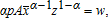 and the solutions for the means of profit, input demand, and output supply, conditional on (p,w,z), are
 (20)
(20) and
and  to relate the observable variables to their conditional means,
  and
and  treat
treat  as observable, and impose the adding-up condition,
 (21)
(21) is realized profit implies pεy=wεx∀(εx,εy). Then the input demand and output supply equations can be written in share form as8
 (22)
(22) (23)
(23) (24)
(24) (25)
(25) is an unbiased complete sufficient statistic, best unbiased for α/(1−α) by the Rao-Blackwell and Lehmann-Scheffé theorems, and maximum likelihood for the marginal distribution for sx conditional on (p,w).9 The invariance principle for maximum likelihood estimators implies that
  is maximum likelihood for α, and therefore CAN and efficient (i.e., it attains the Cramér-Rao lower bound). Because
  by Slutsky's theorem,
  also is efficient. Similarly, conditional on {pt,wt}, the sample mean of output shares has the asymptotic distribution
  Since
Since  Slutsky's theorem implies
  By adding up,
  and the two estimators are equivalent.
 so that
  is unobservable and π is a random variable. Observed profit now is related to expected profit by
  where επ is a random error. Adding up implies py−wx=π by definition. But if
  and
and  as before, then επ=pεy−wεx and the difference on the right of the equals sign does not vanish in general.1025 AGEM is one motivation for this model.11 In that case, the random production function is
 (26)
(26) (27)
(27)Any single equation can be used to identify (α,β) by nonlinear least squares (NLS). Any pair of equations efficiently incorporates the cross-equation parameter restrictions and covariance properties of the error terms. Because επ=pεy−wεx is an exact linear combination of the input demand and output supply errors, the covariance matrix for all three equations is singular. Consequently, one equation must be omitted to estimate the parameters efficiently with standard methods.12
 (28)
(28) or
or  the endogeneity of profit causes bias and inconsistency. First, the term
  is convex in επ and Jensen's inequality therefore implies that
  Second, α/(1−α) is not the mean of sx given (p,w,π) and 1/(1−α) is not the mean of sy given (p,w,π). The coefficient from a simple linear regression on a vector of ones will be biased due to measurement error in the “regressor,” which should be
  rather than 1. Third, the term on the far right of each equation has a random error in the denominator that depends linearly on the random error in the numerator. Although the joint distribution for (εx,εy) determines the precise nature of the asymptotic limits of
  and
and  it is evident from equation (28) that the standard consistency arguments do not apply.13
 (29)
(29) (30)
(30) (31)
(31) or
or  consistently estimates α and that only one equation can be estimated at a time.
 (32)
(32) For example, if ε∼n(0,σ2) and is statistically independent of (p,w), then
 (33)
(33)A Robust and Parsimonious Approach
 (34)
(34) , are
, are
 (35)
(35) (36)
(36) (37)
(37) When κ=1, λ→0 gives the translog system. When λ=1, the netput is on the left, and one obtains netputs derived from a normalized quadratic when κ=1. More general forms are obtained with other values of κ and λ. We conclude that κ=1 with λ variable is sufficient to nest the translog and normalized quadratic functional forms. Also, estimating the parameter κ would provide a system that is in the spirit of, but distinct from, early Box-Cox applications such as 6 or 3. Our point of departure is that equations (35) and (37) provide consistent parameter estimates in share, netput, or a functional form between these cases, as the data dictates.
Using equations (35) or (37) to consider the essential points from above, if λ is incorrectly assumed to be 1 or 0, inconsistent estimates will be obtained because the error terms will (a) be correlated with the regressors, (b) have nonzero expectation, and (c) be heteroskedastic. In contrast, equations (35) and (37) provides a robust and flexible way to incorporate the error term and to nest these two special cases for the functional form of the dependent variable.
Two Applications
 (38)
(38) (39)
(39)One of the most prominent of U.S. agricultural production data sets, summarized in and extended from 4, is the annual time series for the years 1947–2008 produced and maintained by the Economic Research Service of the U.S. Department of Agriculture (also see 5). The groupings of netputs are: y1=livestock; y2=crops; y3=chemicals; y4=fuels and electricity; y5=feed, seed, and livestock purchases, labeled FSL; y6=hired labor; and the numeraire and omitted netput, y7, is other purchased inputs. Own price indexes correspond to the netput groupings: for example, p1=the price of livestock. This is similar in scope to the data analyzed in 2 but does not include pre- and interwar data.18
We will commonly call the inputs z1=capital, z2=owner labor, and z3=time (exogenous technical change) as fixed or quasi-fixed. Capital and owner labor are plausibly fixed. Furthermore, they are the most difficult variables to obtain input prices for, because one or both are residual claimants. However, the essential difference between considering these variables fixed or just optimizing over the other variables is that it may not be appropriate to use them as instruments if they are endogenous. This issue is developed in the second application, where the data are more aggregated across netputs but less aggregated across firms. For this second application, we use agricultural data for Texas from 29, which consist of a single output and three inputs: capital, labor, and materials for the years 1947–1994 (see also 30). In this second data set, unlike the first, prices are available to us for each input, we constructed an implicit price for output, and we can test whether capital is fixed using these factor prices. In both cases, we estimate the models using GMM but with slightly different moments.
The classic reference promoting nonlinear two-stage least squares (NL2SLS) or GMM over maximum likelihood for Box-Cox estimation is found in 1. However, if one searches for  ), as is typically done by gradient methods, one may violate the condition that Θ is a compact set or that the estimator is in the interior of Θ. To illustrate, consider the case in which all errors are homoskedastic and white noise. Then, (g′TWTgT) is nonlinear least squares, which is minimized for data greater than one at
  , which leads to a zero sum of squared errors with all other parameters zero (α=0, B=0, C=0). If one restricts Θ to λ∈[0,1], then the least squares estimator for λ is likely to be on the boundary—that is,
  . A little-known solution has been proposed by 33, which consists of norming the moment conditions to have the same root and asymptotic properties as the original problem. This is the approach taken here.
Consider the U.S. agricultural data with seven netputs, the number of parameters in equation (38) is as follows: 21 unique entries in the B matrix, 18 entries in the C matrix, 6 in α, and λ, for a total of 46 structural parameters. However, note that we use only one additional parameter over previous translog or quadratic studies using similar data. A system of equations increases the number of moment conditions by multiplying by the number of equations while not increasing proportionately the number of model parameters.
These are storied public use data, useful as a benchmark for our approach to see if share regressions are warranted within a modified AGEM model. Policy issues are ignored beyond the inclusion of all payments to farmers in output prices. A second issue is expectations formation for agricultural producers. Futures prices are not helpful for this purpose when using aggregate annual agricultural production data. The standard approach, adopted here, is to ignore this issue for sectoral data (e.g., 2). However, particularly for livestock, accounting for dynamics and price uncertainty in supply seems warranted. We tried different specifications in the empirical application. The results reported here use the lagged cattle price. This is consistent with rational expectations under a martingale difference assumption on price changes over time.
Appropriate instruments also are required for prices and profit. The instruments used in the U.S. application, in natural logarithms, include lagged output prices, contemporaneous input prices, fixed inputs, lagged profits, the square of fixed inputs, unemployment rates, exchange rates, real interest rates, and real per capita gross domestic product (GDP). A vector of ones is also included as one of the instruments. These instruments appear to provide reasonable estimates, and we did not find strong evidence supporting rejection of the orthogonality hypothesis (see the J-test).
The first column of parameter estimates in table 1 presents the NLSUR estimates of equation (38) for U.S. agriculture, a common estimation approach for these types of models (e.g., 2). Note the “significant” estimate of λ of 0.78, which is closer to the netput than the share specification, but also is statistically different from one at all standard significance levels.
| Parameter estimate | NLSUR | GMM |
|---|---|---|
| λ | 0.783** | 0.8703** |
| (0.025) | (0.038) | |
| α1 | 5394.87 | 15348.7* |
| (1929.87) | (7253.96) | |
| b 11 | 1368.80 | 2488.10** |
| (332.089) | (793.062) | |
| b 12 | −1237.16 | −3781.92* |
| (413.521) | (1554.24) | |
| b 13 | 93.970 | (156.462) |
| (57.357) | (160.691) | |
| b 14 | 119.608 | 563.789 |
| (91.079) | (361.205) | |
| b 15 | 24.665 | 195.380 |
| (63.388) | (179.164) | |
| b 16 | −333.040 | −824.923 |
| (173.509) | (526.344) | |
| c 11 | −1222.44 | −4454.14 |
| (860.548) | (3490.94) | |
| c 12 | −0.102 | −0.177 |
| (0.162) | (0.214) | |
| c 13 | 79.725** | 171.757 |
| (30.598) | (89.907) | |
| α2 | 128.865 | −5224.46 |
| (1486.39) | (5421.24) | |
| b 22 | −2441.52** | 308.685 |
| (867.735) | (3371.83) | |
| b 23 | 316.610* | 816.850 |
| (131.977) | (468.806) | |
| b 24 | −134.386 | −1402.63 |
| (211.433) | (1105.96) | |
| b 25 | 252.141 | 527.901 |
| (140.980) | (374.556) | |
| b 26 | 1015.86* | 3047.77 |
| (450.601) | (1658.61) | |
| c 21 | 3605.89* | 13096.6 |
| (1447.70) | (7979.58) | |
| c 22 | 0.737** | 1.172** |
| (0.238) | (0.340) | |
| c 23 | 322.802** | 837.874** |
| (84.318) | (310.779) | |
| α3 | −848.615* | −2121.32* |
| (331.775) | (1040.72) | |
| b 33 | 23.979 | 161.351 |
| (27.725) | (102.227) | |
| b 34 | −77.795 | −211.106 |
| (39.862) | (143.756) | |
| b 35 | −60.310* | −146.729 |
| (30.107) | (82.241) | |
| b 36 | −138.101 | −326.578 |
| (73.512) | (201.958) | |
| c 31 | 133.694 | 759.003 |
| (195.978) | (655.751) | |
| c 32 | −0.106* | −0.149** |
| (0.043) | (0.053) | |
| c 33 | 14.154 | 23.032 |
| (7.297) | (16.305) | |
| α4 | 676.933 | 1931.61 |
| (444.359) | (1645.40) | |
| b 44 | 691.079** | 2381.36* |
| (246.149) | (1194.37) | |
| b 45 | −9.756 | −174.009 |
| (57.867) | (161.339) | |
| b 46 | 1.766 | −103.047 |
| (122.537) | (357.722) | |
| c 41 | −1015.25* | −3192.99 |
| (414.315) | (1850.13) | |
| c 42 | −0.114 | −0.139 |
| (0.066) | (0.103) | |
| c 43 | −71.647** | −156.265** |
| (18.647) | (58.654) | |
| α5 | −163.586 | −345.279 |
| (324.320) | (642.273) | |
| b 55 | 6.902 | 242.104 |
| (53.567) | (199.404) | |
| b 56 | 84.244 | −115.662 |
| (86.293) | (1518.49) | |
| c 51 | −1083.13** | −3246.73 |
| (381.702) | (1518.49) | |
| c 52 | −0.038 | −0.041 |
| (0.049) | (0.042) | |
| c 53 | −15.283 | −37.295 |
| (9.187) | (19.242) | |
| α6 | −3576.41** | −9687.27 |
| (1293.64) | (4501.82) | |
| b 66 | −575.324 | −1415.14 |
| (330.734) | (923.797) | |
| c 61 | −852.186 | −2004.93 |
| (555.426) | (1833.14) | |
| c 62 | 0.401** | 0.464 |
| (0.123) | (0.148) | |
| c 63 | −21.8266 | −43.282 |
| (20.740) | (49.885) | |
| N=59 | J-statistic= | p-value= |
| 71.1084 | 0.084 |
- a Note: Robust standard errors are in parentheses. * and ** indicate statistical significance at the 0.05 and 0.01 levels, respectively. Variable netputs are numbered 1–6, respectively, for livestock, crops, chemicals, fuels and electricity, purchased feeds, seeds, and livestock, and hired labor. The fixed or exogenous variables are numbered as z1=capital, z2=owner labor, z3=time (see equation (38)).
Table 2 presents elasticities calculated at the sample means (see equation (39)). Though a case can be made for the short-run supply of livestock to have a negative slope in the current livestock price (e.g., 16), it is estimated to be positive here. Note that the crop supply elasticity is negative with a p-value of 0.0014. This finding is pervasive against many formulations and tests and suggests price endogeneity. Hence, the identification strategy that we apply is GMM with the instruments previously discussed.
| Elasticity | NLSUR | GMM |
|---|---|---|
| η 11 | 0.219** | 0.152* |
| (0.049) | (0.064) | |
| η 12 | 0.022 | −0.101 |
| (0.050) | (0.064) | |
| η 13 | −0.007 | −0.003 |
| (0.013) | (0.015) | |
| η 14 | −0.008 | 0.017 |
| (0.014) | (0.019) | |
| η 15 | −0.014 | >0.000 |
| (0.010) | (0.009) | |
| η 16 | −0.139** | −0.101 |
| (0.031) | (0.040) | |
| η 21 | 0.024 | −0.079 |
| (0.041) | (0.053) | |
| η 22 | −0.311** | 0.023 |
| (0.097) | (0.164) | |
| η 23 | 0.031 | 0.043 |
| (0.018) | (0.024) | |
| η 24 | −0.044 | −0.081* |
| (0.025) | (0.040) | |
| η 25 | 0.012 | 0.013 |
| (0.015) | (0.016) | |
| η 26 | 0.047 | 0.096 |
| (0.045) | (0.058) | |
| η 31 | 0.078 | 0.041 |
| (0.068) | (0.080) | |
| η 32 | −0.149 | −0.242 |
| (0.119) | (0.154) | |
| η 33 | −0.289** | −0.261** |
| (0.048) | (0.059) | |
| η 34 | 0.060 | 0.075 |
| (0.038) | (0.050) | |
| η 35 | 0.048 | 0.050* |
| (0.027) | (0.021) | |
| η 36 | 0.077 | 0.097 |
| (0.075) | (0.068) | |
| η 41 | 0.068 | −0.106 |
| (0.093) | (0.127) | |
| η 42 | 0.367 | 0.666* |
| (0.201) | (0.323) | |
| η 43 | 0.085 | 0.103 |
| (0.050) | (0.065) | |
| η 44 | −0.909** | −0.985** |
| (0.101) | (0.129) | |
| η 45 | −0.009 | 0.048 |
| (0.054) | (0.052) | |
| η 46 | −0.086 | −0.013 |
| (0.120) | (0.130) | |
| η 51 | 0.156 | −0.0001 |
| (0.106) | (0.099) | |
| η 52 | −0.162 | −0.165 |
| (0.201) | (0.210) | |
| η 53 | 0.107 | 0.109* |
| (0.055) | (0.043) | |
| η 54 | −0.013 | 0.077 |
| (0.085) | (0.082) | |
| η 55 | −0.245** | −0.265** |
| (0.071) | (0.050) | |
| η 56 | −0.212 | 0.014 |
| (0.134) | (0.105) | |
| η 61 | 0.321** | 0.232 |
| (0.071) | (0.091) | |
| η 62 | −0.136 | −0.270 |
| (0.126) | (0.161) | |
| η 63 | 0.043 | 0.048 |
| (0.033) | (0.030) | |
| η 64 | −0.028 | −0.003 |
| (0.041) | (0.045) | |
| η 65 | −0.046 | 0.003 |
| (0.029) | (0.023) | |
| η 66 | −0.099 | 0.004 |
| (0.108) | (0.108) |
The second column of parameter estimates in table 1 presents GMM estimates, with the second column of table 2 presenting the estimated elasticities. The crop supply elasticities are positive and the input elasticities are negative, with the exception of the sixth category (FSL), which is slightly positive and not significantly different from zero.
However, the essential point is that the GMM estimate of λ is 0.8703 and is significantly different from both one and zero. This means that the both the quadratic and the translog profit function are rejected. However, the evidence is much stronger against the translog or share form (λ=0) than the quadratic.
The second data set, Texas (1960–1993), allows us to consider whether all inputs, including capital, are in long-run equilibrium while also testing for the form of the netput equations. Consider this as a netput model where capital and labor are considered quasi-fixed but may actually be in equilibrium. As in 17, the test we adopt is that these inputs are in long-run equilibrium. If capital (or labor) is considered fixed, then the shadow price of capital (∂π/∂z1) will equal the rental rate on capital Rz1; similarly for labor. When an input such as capital is fixed, the firm has a limited ability to adjust its level in both the short- and the long-run. In this case, the input's rental price does not necessarily represent its marginal contribution to profits or shadow price. Such an input is a valid instrument in a GMM estimation procedure. On the other hand, if an input is quasi-fixed, then the firm has a limited ability to adjust its level in the short run, perhaps due to convex adjustment costs, but can do so over time. In long-run equilibrium, the observed levels of quasi-fixed inputs are their optimal levels, and the rental prices of quasi-fixed inputs must be equal to their shadow prices in the profit function. If an input is quasi-fixed, it will not be a valid instrument in the estimating equations for the variable netputs.
 (40)
(40)There are two additional moments for the test of capital and labor as fixed inputs. The estimate of λ is larger than one, at 1.058 (not shown). However, as before, it is significantly different from zero (shares) and one (netputs). Thus, the netput form seems to be more consistent with the data than the share form.
Moving on to the issue of central focus in this application, the parameter estimates for capital and labor (labeled αK and αL, respectively) indicate that there is marginal evidence that capital is fixed (p-value=0.058), but insufficient evidence to reject that labor is in equilibrium (p-value=0.395), with a joint p-value for a Wald test of 0.149. Therefore, we report in tables 3 and 4 results for output, labor, and materials as variable netputs. The estimate of λ changes little (1.061) from the earlier case with labor and capital fixed. Furthermore, the test results for capital are slightly stronger, supporting capital as a fixed input. Elasticity estimates appear comparable to earlier results for U.S. agriculture.
| Parameter | Estimate |
|---|---|
| λ | 1.061** |
| (0.029) | |
| α1 | −0.024 |
| (0.207) | |
| β11 | 0.000003** |
| (0.000001) | |
| β12 | −0.000003** |
| (0.000001) | |
| β13 | −0.000002** |
| (0.000001) | |
| γ 11 | −1.292* |
| (0.684) | |
| γ 12 | 0.023** |
| (0.003) | |
| α2 | −1.138** |
| (0.400) | |
| β22 | 0.00003** |
| (0.00001) | |
| β23 | −0.000002 |
| (0.000003) | |
| γ 21 | 4.953** |
| (1.180) | |
| γ 22 | −0.007 |
| (0.007) | |
| α3 | −0.136 |
| (0.431) | |
| β33 | 0.000003 |
| (0.000003) | |
| γ 31 | −0.556 |
| (1.072) | |
| γ 32 | −0.017** |
| (0.002) | |
| δ 11 | 1849110** |
| (877087) | |
| δ 12 | −3272.420 |
| (2515.930) | |
| αz1 | 303955** |
| (107898) | |
| J-statistic | 8.688 |
| P-value | 0.122 |
- a Note: Standard errors are in parentheses. * and ** indicate significance at the 0.1 and 0.05 levels, respectively. N=34. Variable netputs are 1=agricultural output, 2=labor, 3=materials. Capital (z1) and time (z2) are treated as fixed or exogenous. Fixed capital is tested using αz1. Instruments are real GDP, interest rate, exchange rate, net exports, log profit, and the lag of log profit.
| Elasticity | Estimate |
|---|---|
| η 11 | 0.850** |
| (0.262) | |
| η 12 | −0.048 |
| (0.087) | |
| η 13 | −0.259 |
| (0.293) | |
| η 21 | 0.311 |
| (0.402) | |
| η 22 | −1.039** |
| (0.291) | |
| η 23 | 0.741* |
| (0.418) | |
| η 31 | 0.436 |
| (0.470) | |
| η 32 | 0.294* |
| (0.151) | |
| η 33 | −0.311 |
| (1.105) |
We can see a clear motivation for our approach by contrasting own-price elasticities from the share, netputs, and unrestricted models. Across the various entries in table 5, the sizes and signs of the unrestricted elasticity estimates appear superior from the point of view of optimizing economic behavior. For both the U.S. and Texas data, similar to the point estimates for λ, the unrestricted elasticity estimates are typically much closer to the quantity-dependent estimates than they are to the share-dependent estimates. The latter functional form, that is, the translog, is ubiquitous in the production economics literature. For example, a search on Google Scholar for “translog profit” reveals 643 articles in the first nine months of 2012. This suggests to us that past implicit, perhaps even inappropriate, restrictions on functional form in agricultural netput systems may have had profound implications on the profession's accepted views of important price responses in U.S. agricultural production.
| Netput | Share | Quantity | Unrestricted |
|---|---|---|---|
| A: U.S. agriculture | |||
| Livestock | 0.840 | 0.013 | 0.152 |
| (0.127) | (0.042) | (0.064) | |
| Crops | −0.349 | 0.187 | 0.023 |
| (0.101) | (0.187) | (0.164) | |
| Chemicals | −0.774 | −0.131 | −0.261 |
| (0.078) | (0.049) | (0.059) | |
| Fuel and electricity | −1.051 | −0.967 | −0.985 |
| (0.137) | (0.135) | (0.129) | |
| Feed et al. | −0.230 | −0.286 | −0.265 |
| (0.054) | (0.049) | (0.050) | |
| Hired labor | −1.117 | 0.103 | 0.004 |
| (0.152) | (0.102) | (0.108) | |
| B: Texas agriculture | |||
| Output | 2.747 | 0.765 | 0.850 |
| (3.209) | (0.214) | (0.262) | |
| Labor | −0.471 | −0.464 | −1.039 |
| (1.371) | (0.270) | (0.291) | |
| Materials | −4.650 | −0.427 | −0.311 |
| (3.613) | (1.567) | (1.105) | |
- a Note: Standard errors are in parentheses.
Conclusion
In this article, we have considered rational models of production in the spirit of 25. Given additive errors, models that are incorrectly specified using shares or netputs lead to inconsistent parameter estimates when conventional methods are applied. Hence, a robust specification and estimation procedure is proposed. This approach is able to nest shares or netputs in a simple form. An application to U.S. and Texas agriculture rejects the translog profit function using shares and additive errors. There is weaker (but still quite convincing) evidence that a normalized quadratic profit function using netputs also is inappropriate. This implies that a functional form that is more flexible than either choice, which are most common in the literature, is a preferable econometric model.
We conclude with a few caveats and cautions. When one focuses on one potential improvement in methods while maintaining a host of other assumptions, results may be heavily dependent on what is maintained. For example, for the U.S. sectoral model, we have maintained fixity of capital and owner labor inputs and treated technical change as exogenous while using a novel approach to error specification. Either of these maintained hypotheses may fail under further analysis (10; 31). However, with our robust error specification using Texas data, we find some evidence for rejecting long-run equilibrium in favor of fixed capital, as was also found by 17. Addressing endogenous technical change and a more thorough inquiry that distinguishes errors that are known and unknown by decision makers and econometricians (9; 32) within our framework is a subject of future research.
Supplementary Material
Supplementary material is available at online http://ajae.oxfordjournals.org/.
Appendix
 (41)
(41) (42)
(42) (43)
(43) (44)
(44) (45)
(45) (46)
(46) where the tilde represents nominal profit, the (N+1)-vector of nominal prices, and the (N+1)-vector of random error terms. Because
  and
and  are both homogeneous of degree one in
  ,
,  where p=[p1/pN+1⋯pN/pN+1]′. Note that
  being homogeneous of degree one implies that netputs satisfy the adding up property.
 and
and  where σi=[σi1⋯σiN]′ is the ith row (or column) of Σ.
 ,
,  , and φxy=pwσxy, then OLS on either wx=(α/(1−α))π+wεx or py=(1/(1−α))π+pεy is efficient. In all cases, these results require that
  is not measured with error and is independent of (εx,εy). This hypothesis is testable (13; 19) and warrants serious consideration (11).
 and
and  and
and  , and assuming the joint distribution for (εx,εy,επ) has linear conditional means, the conditional density function for επ is symmetric, and profit is positive. Under these conditions,
  ,
,  ,
,  and
and  is a convergent Taylor series,
  . These properties together give
  ,
, 
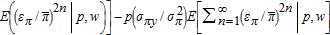 . The first term in square brackets on the right side of both conditional means exceeds one, and the second term has sign opposite to the corresponding covariance term, σπx or σπy, respectively. Subtract the first term in E(sx|p,w) from the first term in E(sy|p,w) to obtain
  . Then sy−sx=1 implies
  which also can be obtained from
  . For example, if σπx<0 (a plausible condition, see equation (26)), both terms on the right in E(sx|p,w) are positive and affect it in the same direction. The negative impact of the second term on the right in E(sy|p,w) therefore must be sufficiently negative to offset the positive bias of the sum of the first term in the conditional mean of the output share plus both terms in the conditional mean of the input share. A converse argument applies to σπy<0. However, more complete or precise statements do not appear possible even in quite simple special cases.
 is used in place of
  , i=1,…,N. An alternative but more cumbersome computation would be to calculate the derivative above at each data point and average them. A reviewer has pointed out that profit is endogenous and one must be careful about assuming that the mean of data is also fixed, as is commonly done in the delta method approach to standard errors. Calculations using average prices and z's exclusively change the standard errors only slightly. However, these prices and z may also be endogenous.