
Statistical evaluation of calcium carbonate equilibrium in natural water
†Correspondence address.
Abstract
A simple statistical model for the Langelier Saturation Index has been developed for all drinking water intakes supplying Cracow. The model has been tested by comparison with the solution of the set of equations governing calcium carbonate equilibria. A high degree of agreement with the results of calculations was achieved, including not only the ionic strength of water solutions but also the so-called ion-pair effects. The model is summarised by simple formulae, which can be used for manual calculation of the Langelier Saturation Index.
INTRODUCTION
The carbon dioxide–carbonic acid equilibrium shifts the pH of rainwater that has not been artificially acidified. Storm water comes into contact with various components of the soil, among which calcium carbonate is one of the most important buffering components. The tendency of water to precipitate or dissolve calcium carbonate is favoured, respectively, by positive and negative values of the Langelier Saturation Index (LSI), which is defined as the difference between the measured water pH and pHS (the pHs is the pH value for which the calcium carbonate is in equilibrium). The Langelier Saturation Index is one of the main parameters that was investigated to evaluate the corrosive properties of water with respect to concrete and steel. In natural water systems, calcium carbonate equilibria are also important because undersaturation and lack of available calcium may result in the mobilisation of heavy metals from soil and sediments. Aggressive waters require special attention in the design of bridges and dams. Despite the fact that the first formulae for the Langelier Saturation Index were developed several decades ago ( Langelier 1936; Rosum & Merrill 1983), new developments are still in progress, as engineers have found the accuracy of calculations to be of great importance in many technical applications. For example, neither unsaturated nor highly-saturated calcium carbonate waters protect water distribution systems against corrosion. Waters that are unsaturated produce calcium-containing protective scaling, while highly saturated waters result in layers that are highly porous, have low resistance to oxygen diffusion, and which may be easily damaged by water hammers in pipeline systems. As calcium forms several inorganic complexes in water, as well as the bicarbonate and carbonate species in the main equilibria reactions, precise calculations require computer-based solutions. Pisigan and Singley (1985) developed statistical formulae for calculating the pHS of many rivers in Florida and now this approach is investigated for the surface waters used for the drinking water supply of Cracow, south Poland. The notation used in the equations is summarised in Appendix I.
METHODS
Main parameters
Statistics are a powerful tool for planning experiments and interpreting results. However, to avoid producing misleading formulae when approximating physical phenomena with statistically elaborated equations, all important parameters should be determined and the relations between them well-understood on the basis of chemical equilibria or physical properties. In the case of investigating calcium carbonate equilibria, the parameters for water that are to be included in the statistical model are the same as those appearing in the set of equations describing the physical model. These parameters were divided here into two groups, the first including the main parameters to which the pHs is the most sensitive, and the second including parameters with a lesser impact on pHs. When defining the first group of parameters, it was temporarily assumed that the effects of inorganic complexes may be ignored, so the carbonic acid equilibrium in water is described by the following set of equations ( Benefield et al. 1982 ; Pankow 1991):

where K1 and K2 are first and second order carbonic acid dissociation constants, respectively; fm and fd are, respectively, the mono- and divalent ionic activity coefficients assumed to be independent of the individual properties of ions; AlkT is the total alkalinity of the water (M); Kw is the water equilibrium constant (M2); [H2CO3*] = [CO2] + [H2CO3]; and [H3O+] = [H+] + [H3O+] + [H5O2+].
Assuming that the concentration of calcium, total alkalinity and pH are known, then equations 1–5 describe the carbonic acid equilibrium of the unknowns [OH–], [HCO3–], [H3O+], [CO32–] and [H2CO3*]. When considering the calcium carbonate equilibria, equations 1–5 are to be supplemented by equation 6 and the concentration of ions [HCO3–], [H3O+], [CO32–] and [OH–], which are recognised to be equal to the ions in equilibrium with calcium carbonate: [HCO3–]eq, [H3O+]eq, [CO32–]eq and [OH–]eq:
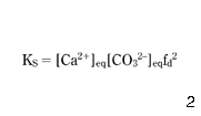
where KS is a solubility constant for CaCO3.
From equations 1–6, the equilibrium pHs with calcium carbonate may be calculated if the impact of inorganic complexes is neglected. As all equilibrium coefficients depend on the temperature and activity coefficients for the ionic strength of water, the main parameters to be included in the statistical formulae are those existing in equations 1–6, plus temperature and total dissolved solids (TDS) or electric conductivity. Either one of the last two mentioned parameters is necessary to calculate the ionic strength of the water solution. Finally, the basic parameters of the statistical models were chosen as [Ca2+], AlkT and TDS. Certainly, temperature (T) has a large impact on the equilibrium, but as separate statistical formulae have been developed for different temperatures, it is not listed here among the main parameters of the statistical model.
Additional parameters
Calcium ions mostly form the following inorganic complexes: [CaOH]+, [CaHCO3]+, [CaCO3]0 and [CaSO4]0 but bicarbonate and carbonate ions are also involved in some other complexes, mostly: [MgHCO3]+ and [MgCO3]0 ( Stumm et al. 1981 ; Benefield et al. 1982 ). To calculate pHs precisely, these complexes in the water solution should be taken into consideration, and finally the concentration of magnesium and sulphate ions were selected as additional parameters.
Form of the equation
From equations 1–6, the following formula for pHs results ( Benefield et al. 1982 ):
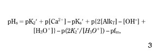
where p is {-log}; K2′ = K2/fd; and Ks′ = Ks/fd2. In the pH range 6.5–9.5, the following approximation of equation 7 is valid ( Benefield et al. 1982 ):
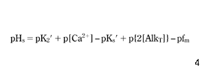
In contrast to equation 7, equation 8 expresses pHs in an explicit form, because on the right hand side there are neither concentrations of hydrogen nor hydroxide ions, therefore pHs may be calculated directly. In equation 8, pHs varies linearly with the logarithm of the concentration of calcium and the logarithm of alkalinity. If, for a narrow temperature range, a linear relationship between K2′, Ks′ and T could be assumed, pHs would also vary linearly with the logarithm of T. Finally, with the exception of TDS, which has a more complex impact, the equilibrium pHs is approximated by a linear combination of logarithms of all the other main parameters. Concluding, a logarithm model was chosen from among several proposals known from the literature ( Pisigan & Singley 1985). For both the main and additional parameters:
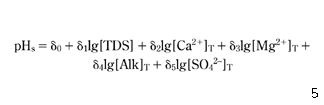
where δ0–δ5 are coefficients that are specific for the given lake or river or, as we will see later, sometimes for a given region with similar geology.
Numerical model
To predict the statistical equations for calcium carbonate equilibrium in water, a numerical program has been developed to solve equation 7, in which the concentration of calcium ions [Ca2+] and the total alkalinity AlkT are determined after the subtracting ions involved in inorganic complexes:
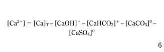
where [Ca]T (total concentration of calcium) is known from chemical analysis.
Equation 4, which calculates the total alkalinity, is applicable exclusively to water with a very low concentration of organic acids (OA–), nitrogen ammonia ions (NH4+) and other ions contributing significantly to the alkalinity of some natural waters ( Schock 1990):
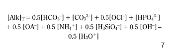
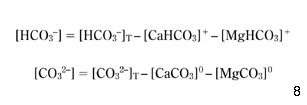
However, for all waters considered here, the concentrations of HPO42–, NH4+, H3SiO4– and OA– were negligible. Finally, in the numerical model, equation 4 has been used, but still, the total alkalinity (AlkT) that appears in equation 7 has to be modified, taking into consideration the inorganic complexes CaHCO3+, MgHCO3+, CaCO30 and MgCO30, which decrease the concentrations of [HCO3–] and [CO32–] available ions in the solution:
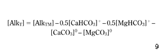
If AlkTM is the value of the total alkalinity that was measured in the water and denoted previously by AlkT, then if the left-hand side of equation 4 is used in equation 7, the following substitution results directly from equations 4, 12 and 13:
To apply equations 10 and 14 to the numerical model, it is necessary to calculate the concentrations of the CaHCO3+, MgHCO3+, CaCO30, MgCO30 and CaSO40 complexes, which has been carried out based on the following equilibria equations ( Truesdell & Jones 1973; Benefield et al. 1982 ).
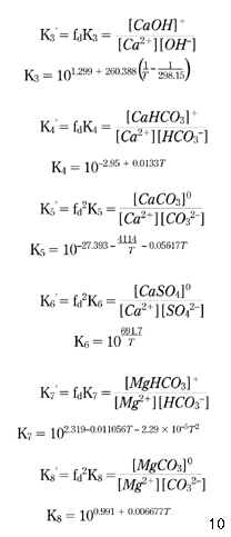
First, making use of equations 10 and 15–20, the concentration of Ca2+ available for the calcium carbonate equilibrium described by equation 7 may be expressed by equation 21:
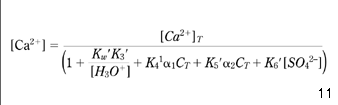
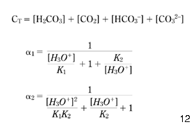
where α1 and α2 denote the parts in which total inorganic carbon (CT) appears as HCO3– and CO32–, respectively (as shown in eqns 22 and 23; Stumm & Morgan 1981; Benefield et al. 1982 ; Pankow 1991):
Second, the total alkalinity AlkTM may be adjusted to AlkT according to equation 14 and, finally, equation 7 may be used to calculate the pHs of the calcium carbonate equilibrium. In this way, the impact of the calcium inorganic complexes on both the concentration of available calcium ions and on the total alkalinity is taken into consideration. To solve equations 7, 14 and 21 with the complementary formulae 15–20 and 22–24, a numerical program was developed. The computations are rather simple and there is no need to describe them here in detail. However, it is worth mentioning that the Davies formula (eqn 25) was used for the activity coefficients, as the ionic strength of the water solution was well below 0.5M in all calculations:
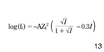
where A = 1.82 × 10⁶ (E × T)–1.5; E = {60954/(T + 116) }-68.937 ( American Public Health Association 1989); T is temperature (K); Zi is the valence of ion i; I is the ionic strength of the water (M).
Statistical equations
The numerical model that was presented in the previous paragraph was used for predicting the pHs of the calcium carbonate equilibrium in waters supplying Cracow from the Raba, Rudawa, Dłubnia and Sanka rivers. Then, one of several statistical equations suggested originally for the rivers of Florida ( Pisigan & Singley 1985) was chosen for application to the main raw water supplies for Cracow.
It was decided that the statistical equation should include all the main parameters listed in the first paragraph of this paper and should satisfy the linear relationship between pHs and the logarithms of the calcium concentration and the total alkalinity, as suggested by equation 7. Based on this, equation 26 was selected:
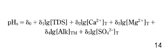
where δ0–δ5 are empirical parameters and the subscript T denotes concentrations known from the chemical analysis of water. The correlation between values of pHs, determined once from equation 7 and once from equation 26, is presented in Fig. 1.

Comparison between chemical equilibria (values from equation 7) and the empirical formula (from equation 26). (——), Regression, 95% confidence.
Equation 26 was used once for all raw water sources supplying Cracow and once separately for each of the rivers. Each time, the empirical coefficients δ0–δ5 were determined by multiple regression analyses and the statistical correlation was evaluated by the coefficient of multiple determination (R2) and the number of data. As the impact of inorganic complexes on calcium carbonate equilibrium is usually limited, a simplification (equation 27) of equation 26 was used in calculations and the results were compared:
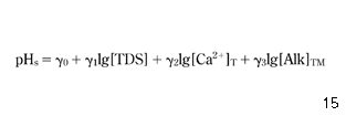
where γ0–γ3 are empirical parameters.
RESULTS
Making use of the results of chemical analyses delivered by the water works company in Cracow from 1994 and 1995, the values of pHS were calculated from the numerical model, including the ion-pair effect (eqns 7,14,21,15–20 and 23–25). The results of the calculations are presented in Table 1 for the same temperature (25°C). Similar calculations were carried out at 5, 10, 15 and 20°C. By using the mean square method, the coefficients δ0–δ5 of equation 26 were calculated from the pHS values resulting from the numerical model. The numerical model was applied to a total of 60 samples that were collected once a month from all four rivers investigated in the present study. Examples of the results of calculations for a temperature of 25°C (298.16K), according to (i) equation 26 and (ii) the numerical model are shown in Table 2.
| Raba | Rudawa | Dłubnia | Sanka | |
|---|---|---|---|---|
| Month | River | River | River | River |
| January | 7.77 | 7.21 | 7.2 | 7.33 |
| February | 7.76 | 7.18 | 7.19 | 7.35 |
| March | 7.73 | 7.22 | 7.18 | 7.42 |
| April | 7.85 | 7.23 | 7.18 | 7.49 |
| May | 7.86 | 7.24 | 7.17 | 7.32 |
| June | 7.85 | 7.25 | 7.16 | 7.34 |
| July | 7.79 | 7.26 | 7.24 | – |
| August | 7.78 | 7.28 | 7.25 | 7.63 |
| September | 7.77 | 7.25 | – | 7.29 |
| October | 7.8 | 7.15 | – | 7.28 |
| November | 7.76 | 7.19 | 7.17 | 7.37 |
| December | 7.77 | 7.2 | 7.17 | 7.4 |
| Month | Raba River | Rudawa River | Dłubnia River | Sanka River | ||||||||
|---|---|---|---|---|---|---|---|---|---|---|---|---|
| (1994) | A | B | C | A | B | C | A | B | C | A | B | C |
| January | 7.77 | 7.77 | 0.00 | 7.21 | 7.21 | 0.00 | 7.20 | 7.20 | 0.00 | 7.33 | 7.33 | 0.01 |
| February | 7.76 | 7.75 | 0.01 | 7.18 | 7.17 | 0.01 | 7.19 | 7.19 | 0.00 | 7.35 | 7.33 | 0.02 |
| March | 7.73 | 7.73 | 0.00 | 7.22 | 7.22 | 0.00 | 7.18 | 7.18 | 0.00 | 7.42 | 7.42 | 0.01 |
| April | 7.85 | 7.85 | 0.00 | 7.23 | 7.23 | 0.00 | 7.18 | 7.18 | 0.00 | 7.49 | 7.49 | 0.00 |
| May | 7.86 | 7.85 | 0.01 | 7.24 | 7.24 | 0.00 | 7.17 | 7.16 | 0.01 | 7.31 | 7.31 | 0.00 |
| June | 7.85 | 7.84 | 0.01 | 7.25 | 7.25 | 0.00 | 7.16 | 7.16 | 0.00 | 7.34 | 7.34 | –0.01 |
| July | 7.79 | 7.79 | 0.00 | 7.26 | 7.26 | 0.00 | 7.24 | 7.23 | 0.01 | – | – | – |
| August | 7.78 | 7.78 | 0.00 | 7.28 | 7.28 | 0.00 | 7.25 | 7.25 | 0.00 | 7.63 | 7.63 | –0.01 |
| September | 7.77 | 7.76 | 0.01 | 7.25 | 7.25 | 0.00 | – | – | – | 7.29 | 7.29 | 0.00 |
| October | 7.80 | 7.80 | 0.00 | 7.15 | 7.15 | 0.00 | – | – | – | 7.28 | 7.27 | 0.01 |
| November | 7.76 | 7.76 | 0.00 | 7.19 | 7.18 | 0.01 | 7.17 | 7.17 | 0.00 | 7.37 | 7.36 | 0.01 |
| December | 7.77 | 7.77 | 0.00 | 7.20 | 7.19 | 0.01 | 7.17 | 7.16 | 0.01 | 7.40 | 7.40 | 0.00 |
- A, pHS as calculated by using equation 7; B, pHS as calculated by using equation 26; C, difference between A and B.
As shown in Tables 2 and 3, the empirical equation 26 fits perfectly to the numerical solution of the equations governing the carbonate equilibria in the surface waters investigated here. When equation 26 was applied separately to each of the rivers, the coefficients δ0–δ5 were calculated by the same method individually for each of the rivers. An example of the results for a temperature of 25°C (298.16K) is shown in Table 4.
| Temperature (K) | δ0 | δ1 | δ2 | δ3 | δ4 | δ5 | R2 |
|---|---|---|---|---|---|---|---|
| 278.16 | 11.327 | 0.231 | –1.011 | –0.009 | –0.985 | 0.068 | 0.999 |
| 283.16 | 11.195 | 0.242 | –1.018 | –0.016 | –0.976 | 0.056 | 0.999 |
| 288.16 | 11.089 | 0.227 | –0.999 | –0.004 | –0.978 | 0.053 | 0.999 |
| 293.16 | 10.948 | 0.207 | –1.012 | –0.004 | –0.945 | 0.061 | 0.998 |
| 298.16 | 10.867 | 0.214 | –1.003 | –0.001 | –0.960 | 0.049 | 0.998 |
| River | δ0 | δ1 | δ2 | δ3 | δ4 | δ5 | R2 |
|---|---|---|---|---|---|---|---|
| Raba | 11.001 | 0.18 | –0.977 | 0.040 | –0.977 | 0.058 | 0.992 |
| Rudawa | 10.867 | 0.209 | –0.907 | 0.046 | –0.899 | –0.040 | 0.997 |
| Dłubnia | 10.947 | 0.273 | –0.903 | 0.009 | –1.104 | –0.011 | 0.993 |
| Sanka | 10.638 | 0.206 | –0.9 | 0.003 | –0.964 | 0.078 | 0.999 |
The fit of pHs, as calculated by using the equations listed in Table 4, was again very good. However, because of a smaller amount of data (15 samples from each river) for R2 it was not possible to prove statistically that the coefficients from Table 4 were more accurate than those from Table 3.
Conclusions
Despite all the uncertainties that result from empirical formulae with statistically predicted coefficients, it was shown that equation 26 may be used for predicting the pHs of a calcium carbonate equilibrium for four rivers supplying Cracow with drinking water. The simple calculations following the formulae listed in Table 3 fitted surprisingly well to precise computer solutions of the set of equations governing the chemical equilibria. All the rivers investigated here are located nearby Cracow, but three of them flow through soil that is rich in calcium and is a good buffer, while the fourth differs in origin. This river originates in the mountains, and is characterised by a much lower alkalinity, even in the place from which the samples were collected.
APPENDIX I
Table A1. Notation used in article
AlkT Total alkalinity of water defined by equations 4 and 14 (M)
AlkTM Total alkalinity predicted from chemical analysis (M) CT Total concentration of dissolved carbonic species fm, fd Mono- and divalent ion activity coefficients I Ionic strength of water (M) KW Equilibrium constant of water (M2) K1, K2 First and second thermodynamic dissociation constants of carbonic acid K3–K7 CaHCO3+ (eqn 16), MgHCO3+ (eqn 19), CaCO30 (eqn 17), MgCO30 (eqn 20), CaSO40 (eqn 18) ionisation constants TDS Total dissolved solids (mg L-1) α1, α2 Fraction of dissolved carbonic species present as HCO3– and CO32–δ0–δ5 Coefficients in the statistical model (eqn 9) γ0–γ3 Empirical parameters in (eqn 27) [OA–] Concentration of organic acids (M)