Out-of-plane static analysis of curved nanobeams resting on an elastic foundation using the method of initial values
Abstract
The unique mechanical properties and versatile applications of curved nanobeams have gained significant attention among researchers, as understanding their mechanical behavior is essential for precise control at the atomic scale. In this study, the out-of-plane static behavior of curved nanobeams resting on an elastic foundation is investigated for small displacements within the framework of nonlocal elasticity theory. Nonlocal constitutive equations are derived and solved using the initial value method, with the approximate transfer matrix approach employed to obtain the principal matrix, ensuring systematic and accurate solutions. A detailed parametric study is conducted to highlight the effects of the nonlocal parameter, opening angle, and elastic foundation interactions on displacements, rotation angles, bending moments, and shear forces. The findings emphasize the critical role of these effects in accurately predicting the mechanical behavior of curved nanoscale structures. The results of this study offer valuable insights for the design and development of curved nanobeam components in nano-engineered materials and devices.
1 INTRODUCTION
In recent years, interest in the mechanics of nanoscale devices and systems has significantly grown as the potential of nanotechnology to address global challenges has become increasingly clear. In particular, devices like biosensors and nanoelectromechanical systems (NEMS) have received considerable attention, as understanding their mechanical behavior has become a primary focus of research for engineers and scientists. Among these nanostructures, carbon nanotubes (CNTs) have gained significant prominence due to their remarkable nanoscale structural and mechanical properties. They can be visualized at the molecular level as tiny hollow cylindrical rods made of graphite-like carbon. Their outstanding characteristics have generated immense interest in the scientific community due to their numerous potential applications. Notably, they possess remarkable resilience, being capable of withstanding stretching along their axis without damage, making them one of the strongest and most flexible materials known. CNTs are estimated to have a Young's modulus of 1 TPa, a tensile strength 29 times greater than that of steel alloys, a current-carrying capacity over 100 times that of copper, and thermal conductivity twice that of pure diamond. Experimental studies on nanotubes have confirmed these theoretical predictions [1-4]. However, experimental assessments of the mechanical properties of such structures is not only time-consuming but also cost-prohibitive, presenting significant constraints. Therefore, research efforts have been directed towards theoretical modeling [5].
Theoretical studies can be broadly categorized into two approaches: atomistic modeling and continuum mechanics. Atomistic modeling employs techniques like molecular dynamics (MD), density functional theory, and tight-binding MD [6-8]. This approach involves analyzing materials at the atomic and molecular levels. However, modeling atomistic details for small-scale structures with a large number of atoms or molecules requires significant computational resources, resulting in time-consuming simulations. Consequently, continuum mechanical modeling constitutes a valuable alternative for analyzing the mechanical behavior of nanostructures. This approach is favored for its greater computational efficiency and more straightforward formulation than previous methods offered. Continuum mechanics can be further classified into classical (local) continuum mechanics and nonlocal continuum mechanics. In classical continuum mechanics, recent studies have investigated the effects of frictional boundary conditions and damping mechanisms on beam and bar dynamics, providing insights into their role in structural stability and vibrational behavior [9, 10].
When dealing with nanoscale structures, consideration of the size effect, which significantly influences their mechanical behavior, is imperative. Classical elasticity theory, being scale-independent, falls short in predicting size effects and is thus inadequate for analyzing nanoscale materials. Consequently, new theories have emerged that incorporate parameters accounting for small-scale effects. Widely adopted theories in nanoscience include nonlocal elasticity, strain gradient theory, surface effect theory, and couple stress theory, with extensive research conducted based on these frameworks [11]. Barretta et al. provide comprehensive summaries of recent developments in modeling and analyzing nanostructures [12]. Among size-dependent continuum mechanics models for nanostructure analysis, the most popular approach is nonlocal elasticity theory. This theory posits that the stress at a point is a function of the strains at all points in the continuum. In this framework, the fundamental equations involve spatial integrals representing the weighted averages of the contributions from related strain tensors at different points within the body. This incorporation of spatial integrals establishes a direct link to the small length scale effect, forming the basis of a spatial-integral constitutive relationship [13-16]. Many researchers have investigated the static and dynamic behavior of Eringen's nonlocal elasticity models in relation to the bending [17-23] buckling [24-27], vibration [28-31], and wave propagation [32-34] of micro- and nanostructures. Recent studies have extended the application of nonlocal elasticity to the stress analysis of nanoscale multi-phase materials [35] and the modal and stress analysis of rotating blades [36], demonstrating the effectiveness of nonlocal elasticity in capturing small-scale effects and its superiority over classical elasticity approaches.
CNTs have often been assumed to behave as perfectly straight beams or cylindrical shells. However, electron microscopy images frequently reveal that these small structures are not generally straight, but instead exhibit a certain degree of curvature or waviness along their length [37, 38]. Numerous studies have explored the mechanical behavior of curved nanobeams, focusing primarily on their buckling, bending, and free vibration characteristics [39-44]. In recent years, significant research efforts have been devoted to analyzing the dynamic and static behaviors of various curved nanostructures. Among these, structures composed of functionally graded materials (FGMs) have garnered significant attention due to their unique material properties. For example, Ahmadi et al. investigated the free vibration behavior of 2D functionally graded curved nanobeams using Hamilton's principle and the first-order shear deformation theory (FSDT). Their study incorporated nonlocal elasticity theory to account for nanoscale effects and examined the influence of material gradation, boundary conditions, and geometric parameters on the nanobeams' natural frequencies and mode shapes [45]. Draiche et al. developed an integral higher-order shear and normal deformation theory (IHSNDT) to analyze the static bending behavior of FG sandwich curved beams, using a hyperbolic cosine stress distribution to satisfy boundary conditions without correction factors and employing Navier's method for the solutions [46]. Hosseini et al. analyzed the free vibration of shallow and deep FG nanobeams using the nonlocal Timoshenko beam model, focusing on how curvature, nonlocal parameters, and material gradation significantly influence vibration frequencies [47]. Vinh et al. examined the free vibration of FG doubly curved nanoshells using a modified first-order shear deformation theory with variable nonlocal parameters to explore the mechanical behaviors of various shell geometries, such as flat plates and cylindrical shells, and investigated the effects of material gradation and geometric ratios on vibration responses [48]. Khater proposed a comprehensive model for curved nanobeams, incorporating beam curvature and surface energy effects using Gurtin–Murdoch surface stress theory combined with Euler–Bernoulli beam theory [49]. Similarly, Manickam et al. investigated the static bending behavior of curved nanobeams reinforced with graphene platelets (GPLs) using a nonlocal nonlinear finite element model. Their study considered the effects of curvature, slenderness ratios, and material gradation, incorporating Eringen's nonlocal elasticity theory for size-dependent modeling [50].
Among the various numerical and semi-analytical methods for solving initial and boundary value problems, the differential transformation method (DTM), finite element method (FEM), differential quadrature method (DQM), and initial value method (IVM) have been demonstrated to be highly effective tools for analyzing the mechanical responses of nanostructures under diverse environmental and loading conditions. Numerous studies have employed DTM [51-54] and DQM [24, 55] to analyze the mechanical properties of single-walled carbon nanotubes (SWCNTs), while similar efforts have focused on double-walled carbon nanotubes (DWCNTs) [56, 57]. Recent studies have further extended these methods to more complex nanostructures and composite systems. For instance, Katiyar et al. employed the FEM to analyze the static bending, buckling, and dynamic behaviors of bidirectional FG plates [58]. Similarly, Cigeroglu employed DQM to study the vibrational characteristics of curved DWCNTs, incorporating geometric and van der Waals force nonlinearities [59]. In another study, Kumar applied the DTM to model the vibrational properties of DWCNTs under various boundary conditions, considering the influence of Winkler elastic foundations on vibration frequencies [60]. Artan and Tepe explored the mechanical behavior of curved SWCNTs using the IVM based on nonlocal elasticity theory [61]. Tufekci et al. performed a static analysis of circular nanobeams using nonlocal elasticity theory. They employed the IVM to obtain exact analytical solutions in cylindrical coordinates and showed that non-local effects and geometric parameters have a significant impact on nanobeam behavior [62]. They further investigated nanobeams with variable curvature and cross-sections, demonstrating how nonlocal parameters influence their mechanical response [63].
A limited number of studies has focused on the mechanical behavior of curved nanobeams resting on an elastic foundation. In the present study, a novel approach was introduced to best approximate the displacements, rotations, and stress resultants of curved nanobeams resting on elastic foundations. The method employs the IVM and matricant approach within the framework of nonlocal elasticity theory, specifically for small displacements and out-of-plane loading conditions to systematically analyze the effects of nonlocal parameters, opening angle, and elastic foundation on the mechanical behavior of curved nanobeams. Traditional methods like DTM, DQM, and FEM, are widely used in nanostructure analysis and have proven effective in various applications. However, FEM and DQM are computationally intensive, while DTM, despite being effective for solving boundary value problems involving various linear and nonlinear equations [64], is constrained by convergence limitations and is only accurate in regions close to the initial conditions [65]. The proposed method provides a computationally efficient and accurate solution, offering a reliable framework for analyzing curved nanobeams and extending the applicability of nonlocal elasticity theory to nanoscale systems.
Recent studies in nonlocal foundation modeling have introduced advanced approaches to address the limitations of the classical Winkler elastic foundation model. Pinnola et al. [66] proposed a hybrid model combining local and nonlocal effects to capture size-dependent behaviors and reaction-driven forces. Similarly, Barretta et al. [67] developed a generalized nonlocal framework to enhance the modeling of nanoscale mechanical interactions. In this study, the elastic foundation is modeled using the Winkler approach, which provides a straightforward yet robust way of representing the local support of the beam. Mechanically, the Winkler model assumes that the reaction force at any point on the nanobeam is directly proportional to its local deflection, idealizing the supporting medium as an array of independent, linear springs. As a result, it enables a systematic investigation into how the interaction between nonlocality, curvature, and elastic support governs the static behavior of curved nanobeams, thereby enhancing the predictive capability of the model for nano-engineered applications. Discussions in the literature have also highlighted certain paradoxes within size-dependent elasticity theory, and several studies have been proposed to address these issues and refine the theoretical framework [68-70]. In our study, the boundary and initial conditions have been carefully defined, and our modeling approach has been structured to align with kinematic and equilibrium boundary conditions. As a result, no “ill-posed” issues of the type discussed in the literature were encountered throughout our analysis. Additionally, the IVM and matricant approach employed in this study solve the equations sequentially and systematically, mitigating potential inconsistencies.
The structure of this paper is organized as follows. In Section 2, the governing equations of a circular nanobeam resting on an elastic foundation are formulated within the framework of nonlocal elasticity theory. In Section 3, a short review of the method of initial values and the ATM approach is presented. The elements of the ATM thereby obtained are presented in the Appendix. A numerical evaluation is performed in Section 4, focusing on the effects of the small-scale parameter, the opening angle on displacement ratios, and the spring constant . Finally, concluding remarks are given in Section 5.
2 GOVERNING EQUATIONS OF THE CIRCULAR NANOBEAM RESTING ON AN ELASTIC FOUNDATION IN NONLOCAL ELASTICITY
3 THE METHOD OF INITIAL VALUES AND THE APPROXIMATE TRANSFER MATRIX
This feature allows us to divide the interval between 0 and into the desired number of segments, facilitating sequential progress towards the opposite end and rapidly improving convergence. If the matricant is known, the solution of the IVP at can be easily determined. The IVM efficiently addresses static indeterminacy by systematically propagating the initial values of displacements, rotations, and stress resultants along the curved beam. The matricant approach allows the solution domain to be divided into smaller intervals, ensuring both faster convergence and high accuracy. The determination of the principal matrix for IVM with the aid of the matricant approach thus provides a precise and consistent methodology for analyzing nanostructures.
The numerical method utilized in this study, which combines the IVM with the ATM approach, has been extensively validated in the literature for solving a variety of structural problems, including those governed by nonlocal elasticity. Previous investigations have demonstrated that this method converges reliably to the solution of nonlocal problems. For example, Eroğlu and Ruta [73] derived approximate closed-form solutions for the vibration analysis of nano-beams with a local/nonlocal mixture, while Eroğlu [74] confirmed the convergence of a perturbation approach based on Eringen's local/nonlocal constitutive equation in one-dimensional structures. These references, along with additional supporting material available in Mathematics in Science and Engineering (vol. 16, Supplement C), substantiate the convergence of the employed technique [75]. Thus, the stabilization observed in our numerical results is a clear indication of the method's robustness and its ability to accurately capture the mechanical behavior of curved nanobeams within the nonlocal elasticity framework.
4 NUMERICAL EVALUATION
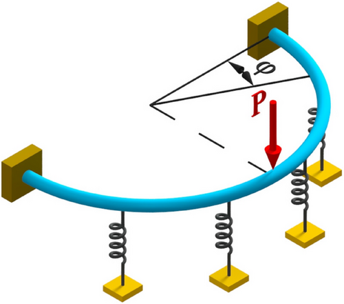
In this study, the circular bar on an elastic half plane clamped at both ends and loaded by a concentrated force at its midpoint resting on an elastic foundation is solved within the framework of nonlocal elasticity (Figure 1).
If we substitute these initial values into Equation (21) and use the boundary conditions and , the other unknown initial values and can be obtained.
The parameters used in this study are as follows: The nonlocal parameter is taken as 1.56 nm [76]. Poisson's ratio and Young's modulus are set to 0.3 and 1 TPa, respectively. The diameter of the circular section is and the length of the rod in the elastic half-plane is . The bending rigidity in the binormal direction is , and the tangential direction bending rigidity is , where is the shear modulus. The concentrated load is N and the dimensionless elastic foundation stiffness is defined as [52, 77, 78].
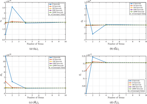
Table 1 and Figure 2 present the convergence behavior of the displacement , rotation , bending moment , and shear force for various numbers of terms and intervals at the point . Here, “” represents the number of terms in the series in Equation (22) and “” the division of the solution interval as described in Equation (23). We observe that using more terms with fewer intervals yields results that are very close to those obtained by using fewer terms with more intervals. However, increasing both the number of terms and the number of intervals significantly increases computation time, thereby reducing computational efficiency. Notably, it was found that after a sufficient number of intervals, the use of more than four terms did not further enhance the accuracy. Therefore, in this study, four terms were used and the solution interval was divided into two segments for an optimal balance of accuracy and computational time, enabling efficient matricant calculation. The elements of the matricant, calculated using Equation (22) with four terms, are provided in the Appendix.
| # of terms | # of intervals | ||||||
|---|---|---|---|---|---|---|---|
| 1 | 10 | 2.0605 | 0 | 6.2383 | 0 | 5.1548 | |
| 1 | 100 | 2.1362 | 0 | 5.1324 | 0 | 5.2016 | |
| 1 | 1,000 | 2.1387 | 0 | 5.0253 | 0 | 5.2060 | |
| 1 | 10,000 | 2.1389 | 0 | 5.0146 | 0 | 5.2064 | |
| 1 | 100,000 | 2.1389 | 0 | 5.0135 | 0 | 5.2065 | |
| 1 | 200,000 | 2.1389 | 0 | 5.0135 | 0 | 5.2065 | |
| 1 | 400,000 | 2.1389 | 0 | 5.0134 | 0 | 5.2065 | |
| 2 | 2 | 3.5715 | 0 | 6.2160 | 0 | 5.2437 | |
| 2 | 4 | 2.6060 | 0 | 5.1050 | 0 | 5.2355 | |
| 2 | 6 | 2.3577 | 0 | 5.0186 | 0 | 5.2223 | |
| 2 | 8 | 2.2644 | 0 | 5.0062 | 0 | 5.2161 | |
| 2 | 10 | 2.2200 | 0 | 5.0049 | 0 | 5.2129 | |
| 2 | 100 | 2.1398 | 0 | 5.0132 | 0 | 5.2065 | |
| 2 | 1,000 | 2.1389 | 0 | 5.0134 | 0 | 5.2065 | |
| 4 | 2 | 2.0543 | 0 | 4.9670 | 0 | 5.2073 | |
| 4 | 4 | 2.1318 | 0 | 5.0135 | 0 | 5.2062 | |
| 4 | 6 | 2.1375 | 0 | 5.0136 | 0 | 5.2064 | |
| 4 | 8 | 2.1385 | 0 | 5.0135 | 0 | 5.2064 | |
| 4 | 10 | 2.1387 | 0 | 5.0135 | 0 | 5.2065 | |
| 4 | 12 | 2.1388 | 0 | 5.0135 | 0 | 5.2065 | |
| 4 | 14 | 2.1389 | 0 | 5.0134 | 0 | 5.2065 | |
| 10 | 2 | 2.1389 | 0 | 5.0134 | 0 | 5.2065 | |
| 10 | 3 | 2.1389 | 0 | 5.0134 | 0 | 5.2065 | |
| 10 | 4 | 2.1389 | 0 | 5.0134 | 0 | 5.2065 | |
| 10 | 5 | 2.1389 | 0 | 5.0134 | 0 | 5.2065 |
4.1 Effects of the small scale parameter
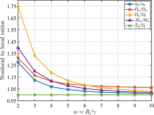
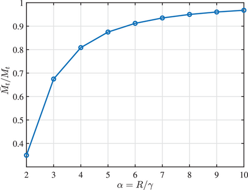
Figure 3 shows the nonlocal-to-local ratios for displacement in the binormal direction, rotation angles about the normal and tangential axes, and bending moment around the normal direction at the angle . It is observed that as increases, the ratios decrease. Notably, the shear force ratio in the binormal direction remains constant. Figure 4 demonstrates that the nonlocal-to-local bending moment ratio around the tangent direction rises with .
4.2 Effects of the angle on displacement ratios
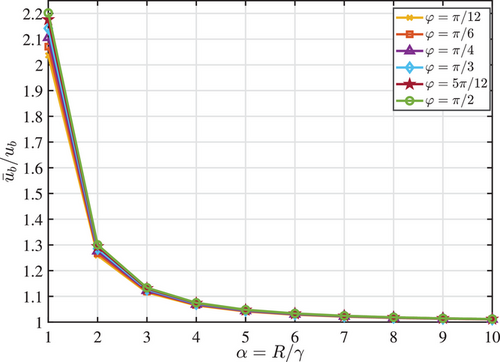
Figure 5 shows the ratio of nonlocal and local displacements as a function of the small-scale parameter for different angles . It can be observed that the results obtained using nonlocal theory diverge significantly from those of the local theory when is small, but this difference decreases as increases. For smaller values of , the ratio changes more noticeably with the angle, but as increases, the influence of the angle reduces, and the results converge. Due to symmetry about the midpoint, the values in the range from to are the same as those from to .
4.3 Effects of the spring constant k on the displacements, rotations, moments, and shear force
Figure 6 illustrates the effects of the dimensionless spring constant and the angle on the nonlocal displacement (), rotation angles ( and ), bending moments ( and ), and shear force (). The nonlocal parameter is fixed at 1.56 nm. In Figure 6a, it is observed that as the angle increases, the displacement also increases, and higher values of spring constant result in larger displacements. The initial condition is confirmed by the graph, indicating zero displacement at . Figure 6b shows that the rotation angle () decreases to a minimum around and then increases. Higher values cause more negative values at the minimum, consistent with the initial and boundary conditions and . In Figure 6c, the rotation angle () continuously decreases to a minimum at . Higher values result in more negative angles, consistent with . Figure 6d shows that the bending moment () increases with . Higher values make this increase more pronounced. Figure 6e demonstrates that the bending moment () decreases to a minimum around and then increases towards . Higher values intensify these changes, consistent with . Finally, Figure 6f shows that the shear force () increases with . Higher values lead to greater changes, consistent with the initial condition . These results are also consistent with the values in Table 1 for at , calculated using the ATM approach with four terms and two intervals. These observations highlight the significant effects of variations in and on the mechanical behavior of the system.
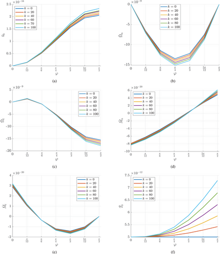
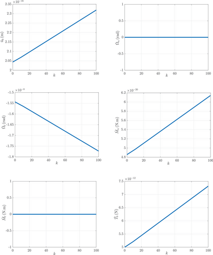
Figure 7 illustrates the effects of the nondimensional spring constant on the nonlocal displacements, rotations, moments, and shear forces at . It can be observed that the displacement , the bending moment in the normal direction , and the shear force both increase with . In contrast, the rotation around the tangent direction decreases with . The rotation and the moment remain constant at zero for all values of , which is consistent with the boundary conditions. When analyzed at and , the graphs are observed to be consistent with the data presented in Table 1.
5 CONCLUSION
This study presents a novel analytical framework to investigate the out-of-plane static behavior of curved nanobeams resting on elastic foundations within the scope of nonlocal elasticity theory. The results highlight the critical role of nonlocal effects in accurately predicting mechanical behavior at the nanoscale. As nonlocal parameters become more prominent, the discrepancies between classical and nonlocal elasticity predictions increase, emphasizing the necessity of nonlocal models for reliable analyses. Additionally, the elastic foundation constant () and angular variations () significantly affect the displacements, rotations, and stress resultants, particularly at smaller angular values. The integration of the IVM and matricant approach provides a systematic, accurate, and effective solution framework that constitutes a practical and robust alternative to conventional approaches in the literature, enabling the precise modeling of curved nanobeams. The convergence analysis validates the robustness of the proposed method, demonstrating that optimal combination of terms and intervals enhances computational efficiency without sacrificing accuracy. Furthermore, the insights gained contribute to the design and optimization of curved beam components in micro-electro-mechanical systems and NEMS, where the accurate modeling of size effects is crucial.
ACKNOWLEDGMENTS
The authors sincerely thank the editor and the anonymous reviewers for their constructive comments and insightful feedback, which have significantly enhanced the quality of the manuscript. This study has been supported by The Scientific and Technological Research Council of Turkey (TUBITAK) with Project Number: 107M341.
CONFLICT OF INTEREST STATEMENT
On behalf of all authors, the corresponding author states that there is no conflict of interest.


