Light detection and ranging measurements of wake dynamics. Part II: two-dimensional scanning
Abstract
A nacelle-mounted lidar system pointing downstream has been used to measure wind turbine wake dynamics. The new measurement and data analysis techniques allow estimation of quasi-instantaneous wind fields in planes perpendicular to the rotor axis. A newly developed wake tracking procedure delivers the instantaneous transversal wake position which is quantitatively compared with the prediction of the Dynamic Wake Meandering model. The results, shown for two 10-min time series, suggest that the conjecture of the wake behaving as a passive tracer is a fair approximation; this corroborates and expands the results of one-dimensional measurements already presented in the first part of this paper. Consequently, it is now possible to separate the deterministic and turbulent parts of the wake wind field, thus enabling capturing the wake in the meandering frame of reference. The results correspond, qualitatively and to some extent quantitatively, to the expectations from CFD simulations which are compared in the paper. Copyright © 2010 John Wiley & Sons, Ltd.
1. INTRODUCTION
The need for full-scale wake experimental data has been increasing in the wind energy community. State-of-the-art wind farm models are in need of development and validation based on more accurate and comprehensive wake measurements. Lately, considerable discrepancies between predicted and measured energy yields of large wind farms have been observed.1 Moreover, attention has also been drawn to dynamic wake effects. These are not only relevant for production estimation but in particular for loading estimation. The so-called wake meandering is detrimental for some components of the wind turbine,2 and a thorough understanding and quantitative estimation of its effects is needed.
Full-scale wake measurements for capturing these dynamic effects are hardly possible with conventional measurement techniques. The high cost and low flexibility of meteorological masts restricts the installation of a sufficient number of measurement points. Traditional wake measurements produce stationary horizontal wind speed profiles at hub height level. In some cases also vertical characteristics can be obtained. The spatial resolution is given by a small number of anemometers from which the wake dynamics cannot be resolved. In contrast to conventional recording techniques, remote sensing instruments can be positioned quickly and provide almost instantaneous measurement at different spatial points with high resolution. In this regard, the light detection and ranging (lidar) technology presents great advantages due to its speed, robustness and flexibility in measuring wind fields. For instance, inflow measurements from the nacelle of a wind turbine have been successfully tested.3,4 In that case the fast measurement at a fixed point in front of the turbine assisted an advanced wind turbine control system.
This paper describes the application of lidar to wind field measurements in the wake of a 95 kW wind turbine. As in the previous example, the lidar system is installed at the nacelle but pointing downstream and implementing more complex scanning. The measurements were performed at a downstream distance of four diameters, which is considered to cover the far–wake regime. This investigation is conceived as a proof of concept of this type of measurement. New analysis techniques are developed to provide data useful for steady and dynamic wake model verification. Part I of this paper5 exposes the first measurement campaign of this type along with the working principles of the instrument. Furthermore, the installation procedure on the wind turbine nacelle at the Risø test field in Roskilde is also explained. Part II of the paper deals mainly with the analysis of the so-called two-dimensional wake measurements. These enable estimation of the wake wind field in cross-sections perpendicular (here also named transversal) to the mean rotor axis and eventually large-scale dynamics of the wake. Here we explain firstly, the two-dimensional wake measurements in detail and the methods developed to capture wake dynamics; secondly, models for dynamic and deterministic wake are exposed and finally compared with two individual measurements.
2. MEASUREMENT SETUP
2.1. Lidar setup
2.1.1. Line of sight wind speed in wake
Lidars measure the so-called line-of-sight wind speed (ulos) which is aligned with the laser beam. Although the beam direction in space is exactly known, it is not possible to deduce the three-dimensional wind speed vector from this single measurement. Three non-aligned measurements aiming at the same spatial point are needed in order to obtain the actual vector. Due to the use of only one beam in this investigation, misalignment of the actual wind and line-of-sight vectors can lead to underestimation of the Euclidean norm of the wind vector (Figure 1). A projection of ulos to the rotor (wake) axis is a possible solution to the problem when averages in time are considered. However, this is dependent on a perfect positioning of the wind turbine rotor with respect to the wind, which is in practice not fully guaranteed. Therefore this sort of correction would introduce some error in the instantaneous wind fields, and consequently only the measured ulos is used for the analysis. Moreover, for the main purposes of this paper, which is the observation of the large-scale dynamics, the measurement of the absolute wind vector is not of primary concern. Therefore this limitation is in this case almost irrelevant.
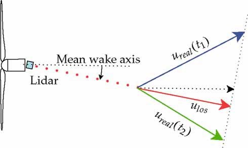
Comparison of measured line-of-sight wind speed (ulos) with instantaneous wind vector.
2.1.2. Sphere scan mode
For this experiment the lidar is located at the rear of the nacelle, the focus distance is fixed while the beam direction is continuously changed. Under these conditions the focus point domain is a surface represented by a patch of a sphere; due to this feature this type of scanning is referenced to as two-dimensional. The scanning mode is achieved by a combined vertical and horizontal independent angular movement of the laser beam. The tilt is performed by optical means, where an oscillating wedge with axis parallel to the beam deviates it following almost vertical arcs. The pan is achieved by moving the whole lidar optical head, including the tilting wedge, to the left and right with an external mechanism. The positioning of the whole mechanical system is recorded at each measurement point. The beam direction is estimated from these signals based on the geometry of the system. A satisfactory accuracy was achieved in the laboratory by observing the movement of the laser beam on a wall. Some more details about the scanning system can be seen in Bingöl et al.5 For the present configuration one pan movement is made in approximately 1.1 s; measurements performed during this time are called a snapshot. During the combined tilt/pan movement of the laser beam, the focus point follows an irregular trajectory as shown by black dots in Figure 2. The path is followed along the arcs beginning either on the left or the right side. This differs from an optimal trajectory where the distribution of the points is more homogeneous over the target area. However, it is considered as the most practical solution at the moment due to limitations in the design of the prototype lidar device. An intentional lack of synchronization between the pan and tilt movements is used as an advantage to cover the whole scan area. In effect, the path followed by the focus point is hardly the same at any pan cycle, thus generating a pattern covering the whole area after some consecutive pan movements.
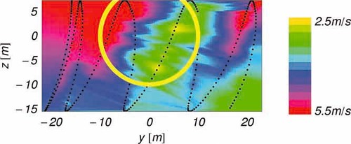
Two-dimensional interpolation of ulos at 80 m (∼4 diameters) behind the turbine. Black dots display the measured (focused) points. Incomplete circle represents rotor projection on the target area. Measurement during ∼1.1 s on 05.07.2006 sometime between 4:00 and 4:10 a.m.
2.2. Wind turbine
The studied wind turbine is the stall regulated Tellus 95 kW which is installed at Risø test field in Roskilde. It has a hub height of 29.3 m and a rotor diameter of 19.0 m. This turbine has been part of different measurement campaigns, and therefore it is suitably instrumented for this research. Some adaptations were performed to the turbine nacelle in order to install the lidar's optical head. A detailed description can be found in Bingöl et al.5 along with the characteristics of the test facilities. Measured operational characteristics such as thrust coefficient and power curve are available from earlier measurement campaigns. The site is relatively flat, and other test turbines are installed and operating nearby. Furthermore, meteorological inflow data are available from a meteorological mast installed close to the turbine.
2.3. Measurement campaign
The measurements analyzed here were performed at a fixed focus distance of 80 m (∼4 diameters). This is well within the range of the lidar, and additionally the wake deficit should be observable for different operational conditions, specially those of operation at high thrust coefficient. At this distance the focus volume extends ∼20 m and has a focal radius of 0.002 m.6 The average maximum geometrical bias in ulos due to misalignment, as explained in section 2.1.1, is an underestimation in the order of 3%.
During the campaign 128-point Doppler spectra of line-of-sight measurements were stored, which each were the result of averaging over 256 spectra measured at a certain area in space. The spectra files, covering a period of 10 min each, contain ∼172 × 103 spectra corresponding to the same amount of focus points during a 10 min recording period. These large number of spectra are post-processed to obtain ulos by means of a centroid procedure.7
Each time series is checked for plausibility of the estimated ulos at each spatial point. Mainly, it is a search for single jumps and spikes, which occasionally appear in the time series. These events represent a wrong estimation of the Doppler spectrum peak, which is most probably a consequence of very flat Doppler spectra due to low backscattering and/or highly turbulent wind.
In the case that a single non-realistic value is found, the wind speed is linearly interpolated between the two neighboring plausible values, i.e. between ulos(ti−1) and ulos(ti+1). This approach has proved to be robust and seems to be adequate, since the two neighboring points are located in space relatively close to each other.
2.4. Selected data
-
Wind directions where the wind turbine is in free flow and not in the wake of its neighboring turbines at the test site.
-
Wind speeds in the range from 4 to 7 m s−1 in order to have a partial power regime with a high thrust coefficient and consequently a clearly observable wake deficit.
-
Doppler spectra with clearly defined peaks. In some cases with high turbulence the spectra look flat, which complicates the wind speed estimation.
Data from 3 days have been analyzed, namely the 3rd and 4th June 2006 and the 5th July 2006, which respectively fulfill the mentioned criteria. During the first and second days a westerly wind direction was experienced, and therefore the reference meteorological mast is undisturbed by the wake flow. On the third day an easterly wind direction was predominant, therefore the meteorological mast was operating in the wake of the wind turbine.
The procedures exposed in the paper were tested on more than 48 hours of measurement during the three mentioned days. Unfortunately the target measurement area was not large enough to cover the whole wake. Moreover, due to topographical effects the wake is shifted vertically in different degree depending on the wind direction sector. This is a rather problematic issue for the westerly measurements (03.06.2006 and 04.06.2006), since the wake was severely cut from above and the wake tracking procedures do not work properly all the time. In order to illustrate the developed procedures, we show in this paper individual results for two measurements on 05.07.2006 where great part of the wake is inside of the target area. The data, which were subdivided in 10 min correspond to the periods from 3:50 to 4:00 a.m and from 4:00 to 4:10 a.m. The meteorological mast is disturbed by the wake at this time, however this issue can be overcome as will be shown. In fact all the undisturbed characteristics needed for the analysis are estimated from the lidar measurements or by filtering the data from the meteorological mast. There was stable atmospheric stratification and the inflow conditions were very similar, however the two time series show different characteristics. During the first 10 min the wind turbine changed its yaw position twice while during the next 10 min the yaw position remained constant. These contrast exposes the ability of the developed methods to track the wake and separate the effects of large scale movements.
3. DATA ANALYSIS
3.1. Quasi-instantaneous wind field
In the scope of this investigation, the above mentioned measuring rate of ∼1.1 s per snapshot (∼0.92 s−1) is assumed as a quasi-instantaneous measurement. The obtained snapshot is made up of ulos measured on an irregular path (black dots in Figure 2), which for convenience is interpolated into a Cartesian grid with regular spacing. A rectangular grid is used with 144 and 112 divisions in the horizontal and vertical directions, respectively.
A Delaunay triangulation is used to interpolate linearly wind speeds in between the irregularly distributed measuring points on the target area. The technique is based first on a triangulation of the area, where the vertexes of the triangles are located at the measurement points. The created mesh is a collection of triangles with non-crossing sides and the least sharp possible angles. In a second step, values at any point on the regular rectangular mesh are obtained by linear interpolation on the triangular plane containing the particular node. The interpolation of a snapshot, using an efficient implementation of this method,8 can be seen in Figure 2. A low wind speed area, exposing an incomplete wake, is observed to the top-right along with expected general features of the wind field. The surrounding undisturbed wind can be seen to the left, whereby also details of the vertical wind shear can be observed.
3.2. Steady wind fields
Steady wind fields are of interest for observing the wind field characteristics without the influence of small scale turbulence. These are obtained by averaging the wind fields in time. At this point it is important to define a proper frame of reference. A wind turbine wake is characterized by large scale meandering movements, which affect the wind field observed from different reference frames.5,9,10 Observing from the ground, at the nacelle or following the wake has an effect on the perceived average wind speed and turbulence. Three different frames of reference can be defined in regards to such measurements as explained below.
Fixed frame of reference.
The frame of reference attached to the ground is called fixed frame of reference. Standing on the ground an observer sees a dynamic wake moving transversally in the vertical and horizontal directions, respectively (i.e. wake meandering). This is analogous to the wind field a set of ground based anemometers would sense if distributed on a transversal area at the same downstream position.
Nacelle frame of reference.
Standing at the nacelle, and focusing at a particular downstream distance, an observed wake deficit will also meander. However, the frame of reference rotates with the yaw system. Therefore, the wind field resolved in this frame of reference can be different from the one resolved in the fixed frame of reference. Consequently, our measurements performed from the nacelle potentially also contain contributions originating from the turbine yaw movement. Moreover, if the turbine does not yaw during the time period of observation, then the captured wake coincides with that resolved in the fixed frame of reference.
Meandering frame of reference.
A convenient redefinition or relocation of the origin of the frame of reference can be done if the actual instantaneous position of the wake is known. It is expected that the meandering effect disappears if the origin is made coincide with a fixed point on the moving wake at every instant. The wake tracking procedure explained in section 3.5 enables defining a meandering frame of reference for the two-dimensional lidar measurements. An average over time of the snapshots can be performed in this frame of reference. In this way it is possible to estimate the quasi-steady wake emitted by the turbine without any large scale atmospheric influence.
3.3. Mean undisturbed wind shear
Mean vertical profiles can be obtained from averaged two-dimensional wind fields measured with lidar, or from meteorological mast measurements if these are performed at different heights simultaneously. However, if the intention is to get the undisturbed vertical wind shear, then there is a limitation when the meteorological mast is in wake at the time of measurement. A possible solution is offered by the lidar measurements. If the scanned area is large enough, such that the wake does not move all around the measured area during the averaging period, then the free shear can be extracted from the unaffected areas of the two-dimensional wind fields (Figure 4).
3.4. Atmosphere–wake interaction
 ). The second is the axisymmetric mean wake deficit (Δu), associated with an uniform inflow with wind speed equal to the wind speed at hub height. The third component is an induction residual due to asymmetric inflow (ϵi), caused for instance by a vertical wind shear. This has a three dimensional character, for example when there is an additional horizontal wind shear. The last component is the total wake turbulence (u′). As a consequence of this approach, the instantaneous stream-wise wind speed can be expressed as in equation (1). Hence, the instantaneous wake deficit with superimposed turbulence can be obtained by direct subtraction of the mean vertical shear from an instantaneous wake recording.
 (1)
(1)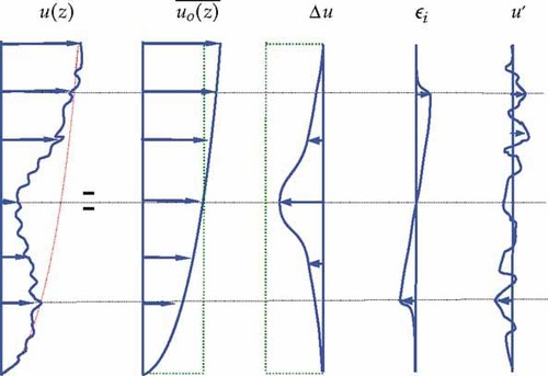
Idealized decomposition of turbulent wind field in wake. Superposition of vertical wind shear, wake deficit, induction asymmetry and total turbulence.
3.5. Wake tracking
The position of a particular point fixed to the wake deficit in a measuring cross-section can be estimated from quasi-instantaneous measurements. Accordingly, it is possible to perform analysis of the time evolution of the transversal wake position. Knowledge of the actual instantaneous position of the wake has two important applications. First, the estimated time series can be used to understand the physics behind the large scale transversal movements of wind turbine wakes and to validate meandering models. Second, as mentioned in section 3.2, the wake can be resolved in the meandering frame of reference. A wind turbine operating downstream of another turbine observes the upstream emitted wake deficit sweeping across the rotor. In consequence, this is of primary importance when estimating wind turbine performance operating in wake.
During this research two approaches were tested for identifying the wake position in a particular two-dimensional wind field (snapshot). Both methods are based on the capability of isolating the wake deficit from the atmospheric wind shear. The aim is to estimate the most likely position of a fixed point in the isolated wind speed deficit, like for instance the deficit center.
The first, and simplest, approach to find the position of the wake is to apply a mass-density analogy. The measured area is assumed to be a plate where the wind speed deficit acts as a non-homogeneous mass. The center of mass of the plate is assumed to be the reference point of the wake position. Unfortunately, initial tests of this approach were not always successful. The method is not robust for two reasons, namely, 1) errors in ulos at some focus points (non cleaned spikes) can bias strongly the estimated wake position. 2) Errors also happen when low wind speed areas exist simultaneously with the turbine wake (right-bottom in Figure 2). This can be caused by nearby wakes or by turbulent structures with characteristic spatial dimensions comparable with that of the wake deficit.
 (2)
(2) (3)
(3) (4)
(4)The selected generic Gaussian function fits even in cases where the wind speed deficit presents asymmetry, inhomogeneity, or even if it is partially contained in the target area. This is of advantage, since in general it is expected that the measured turbulent wind fields display any or all of these characteristics. However, a plausibility check of the fitted function has to be performed in order to find whether a wind field is suitable or not for wake tracking. For instance, in case the wake meanders strongly, just a small part of the deficit could be ‘visible’, and the fitting could be highly unreliable.
3.6. Steady wake in meandering frame of reference
After estimation of the wake position for every snapshot in a 10-min time series, the wind fields (snapshots) are translated to a common center using the estimated instantaneous position (μy, μz)i. The mean wake deficit, expressed in the meandering frame of reference, is obtained by averaging all aligned snapshots, thus eliminating the inherent turbulence contribution to the instantaneous wake wind fields. In other words, it is possible to sort out all turbulent components, namely, the ambient, the wake added, and the apparent meandering turbulence. These depend on different operating conditions, for instance rotor loading conditions, the ambient turbulence intensity, the ambient turbulence length scale, downstream distance, etc. Therefore, it must be noted that the relative contributions of each of these to the total turbulence cannot be generalized.
4. WAKE MODELING
The main application of the measurement techniques developed in this paper is the acquisition of validation data for an engineering model for wake dynamics, namely the dynamic wake meandering model (DWM). The wake modeling is based on the assumption that the wake behaves as a passive tracer.9 Accordingly, the wake can be idealized as a cascade of disks which move transversally (i.e. horizontally and vertically) following large scale eddies in the atmosphere as passive bodies. In order to simulate the wake, two independent models are needed. One for description of the meandering movement and another for the steady wake flow.
4.1. Meandering movement
The transversal movement of each wake disk is assumed to be affected mainly by spatial scales in the order of two rotor diameters and larger.9 In other words, the turbulent structures in the atmosphere, which are smaller than the rotor size, play a secondary role in the meandering process. Therefore, the wake movement can be predicted downstream based on measurements of wind direction and the vertical wind speed near the rotor filtered with a low-pass filter. An explanation of the calculation procedure is found in Part I.5 Eventually two time series of the wake position are obtained, namely, the measured, resolved with the wake tracking algorithm described in section 3.5, and the predicted, based on the meandering model using measurements from a reference meteorological mast. Finally, the similarity between the two time series is quantified by comparison of their cross-correlation.
Single-point inflow measurements are assumed to be reliable for meandering prediction. This is based on the assumption that large scale turbulence, in the order of magnitude of two rotor diameters and greater, should be reasonably correlated over the whole rotor area. This simplification can be made for moderate downstream distances without losing much information on the meandering process.12 The assumption is tested here by comparing the cross-correlation between the tracked wake and the modeled position. Mainly two modeled time series are generated, one using only the wind characteristics at hub height, and another using the average between the last and the measurement at the lower tip height.
4.2. Steady wake
A wake model proposed by Ainslie11 is used for estimation of steady single wakes. In principle, the calculation is performed in the far–wake regime, where the pressure field is assumed to have adjusted to the ambient pressure. The model is based on the assumption of an azimuthally symmetric wind speed deficit around the wake center line. The flow is calculated as a boundary layer flow, where the gradients in directions perpendicular to the predominant flow direction are much larger than the longitudinal gradients, and the pressure gradients are neglected. Hence, the single wake is modeled with two-dimensional Reynolds averaged Navier-Stokes equations (RANS), using a Gaussian wake deficit at two diameters as an approximate initial condition. For the turbulence closure it is suggested to use an eddy viscosity model, which depends on the atmospheric and the wake added turbulence.13 For this experiment simulations were performed with the implementation of this model for single wake calculation in the Farm LAyout Program (FLaP) of ForWind at University of Oldenburg.14
5. RESULTS AND DISCUSS ION
The following results are presented mainly for the wake in the nacelle and the meandering frame of reference. The signal of turbine yaw position was not available during the measurement period. Therefore the calculation of the wind fields in the fixed frame of reference is not possible. However, the results in the two other frames of reference are considered illustrative enough of the capabilities of this new measurement and analysis technique.
5.1. Quasi-instantaneous fields
The interpolation procedure (explained in section 3.1) was evaluated by visual inspection of snapshot sequences for each 10-min time series. The approach works satisfactorily, although some non-optimal effects are observed. As can be noticed in Figure 2 the density of the measured points is higher in the vertical than in the horizontal direction. This particular distribution of points produces triangulations with very thin, horizontally oriented, triangles. This has an important unfavorable effect in the resolution of the detailed wind field but, in our opinion, a rather small effect on the wake tracking method. The fitting procedure of a bivariate Gaussian function, as outlined in section 3.5, is a very robust procedure, which is insensitive to isolated non-optimal estimations. Therefore, for our main purposes the effect is not relevant, and the search for a fully optimized interpolation method was not prioritized. Furthermore, this effect could be readily counteracted or avoided with an improved trajectory and distribution of the measurement points on the scanned area.
5.2. Vertical wind shear
The two-dimensional wind field obtained with lidar, averaged over 10 min (see Figure 7), is assumed to be unaffected by the wake at the left side of the target cross-section. Therefore the vertical mean wind speed profile is estimated from this part of the wind field by averaging on a narrow vertical band around 3 m wide (Figure 4).
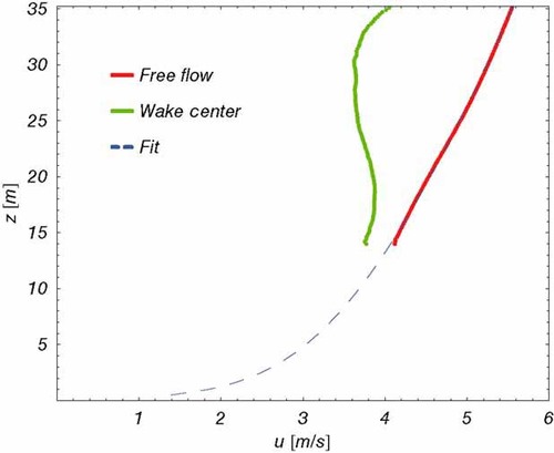
Undisturbed and wake affected vertical wind shear at 80 m (∼4 diameters) behind the turbine. Profiles extracted from 10 min average wind field (Figure 7). Dashed line shows the fit to diabatic vertical profile as defined in equation (5). Measurement on 05.07.2006 from 4:00 to 4:10 a.m.
Fitted wind shear.
 (5a)
(5a) (5b)
(5b)5.3. Wake dynamics
5.3.1. Comparison of measurement and model
The tracked downstream wake position from the lidar measurements were compared with predictions from the DWM model. The required input for this model was obtained from the reference meteorological mast. Two sonic anemometers at 20 m and 30 m (hub height) were available for this purpose. The wind direction signal was filtered by means of a moving average with a predefined filter window equivalent to two diameters. The disk transversal speeds vc and wc (see Part I5) are estimated from this filtered signal. Moreover, the stream-wise advection speed of the wake is set equal to the mean inflow wind speed uT =  .
.
In this case the meteorological mast was positioned in the wake of the wind turbine. Therefore, the mean wind speed ( ) was estimated from the lidar measurement while the wind direction time series was obtained from the meteorological mast. The additional turbulence generated by the turbine is represented by scales in the order of magnitude of the rotor diameter and smaller.16 Consequently, it is hardly possible that the wind turbine will affect significantly the large scale components of the wind direction sensed by the sonics. Consequently, in the context of meandering prediction, it is considered irrelevant whether the wind direction measurements are performed with the meteorological mast in wake or in free flow.
Prediction of meandering was performed with the individual wind direction from sonic at hub height (30 m) as well as with an average between this and the measurement at 20 m. The result for the last is shown in Figure 5. The cross-correlation between the predicted and measured time series has been calculated giving a maximum cross-covariance of ∼0.58. This last value depends on the filtering applied to the input signal in the meandering model. In this case the filtering is dependent only on the window size of the moving average. An analysis of the effect of the window size is shown in Figure 6. The prediction using wind direction from sonic anemometer at 30 m and from average between 20 m and 30 m are compared. The significant change in slope at a window size of the order of two diameters is in agreement with the definition proposed in Larsen et al.9 At this point an inflection is seen, at which the maximum cross-correlation begins to saturate. This suggests the appropriateness of using a cut-off frequency separating large turbulence scales from small turbulence scales in the context of the DWM. Moreover, the relatively small difference between both curves (Figure 6) suggests the suitability of using measurements at one single height.
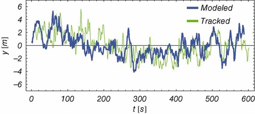
Comparison of predicted and tracked (measured) wake position for a 10-min time series. Prediction with the DWM using average wind direction from sonic anemometers at 20 and 30 m and a window size of two diameters for the running average. Measurement on 05.07.2006 from 4:00 to 4:10 a.m.
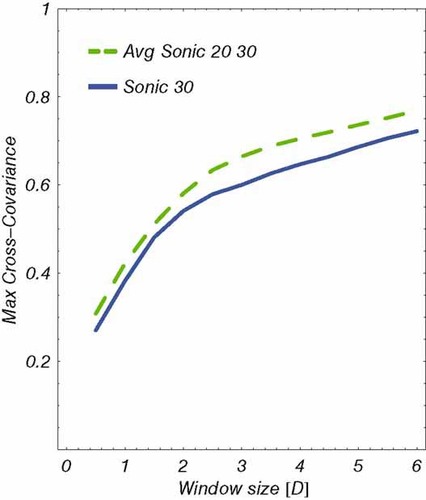
Comparison of effect of filter window size (in rotor diameters) on maximum cross-covariance between measured and predicted meandering. Prediction using wind direction from sonic anemometer at 30 m (solid) and from average between 20 and 30 m (dashed). Measurement on 05.07.2006 from 4:00 to 4:10 a.m.
5.3.2. Robustness of fitting procedure
The fitting procedure is relatively fast with calculation times in the order of magnitude of the measurement speed. This means that for this experiment a snapshot could be fitted in average in around 1 s. However, this speed is strongly dependent on the character of the instantaneous wind field, for instance, pronounced deficits which center is located inside the target area are relatively faster to fit. In fact some snapshots present difficulties to be fitted. Therefore a set of plausibility criteria were devised to pick out unreliable data (see Table I). The limit values for each independent parameter were defined as follows: the position of the wake center (yc, zc) was restricted to the target area; the characteristic width (σy, σz) is assumed valid only if it does not exceed a value of one and a half turbine radius (1.5ℜ). The definition of a limit value for the scaling A could not be done a priori. Therefore, statistics of the obtained values were used to estimate a valid range. A top limit based on the 75th percentile was defined due to high variability of the values. In consequence, values higher than 30,434, were selected as wrong for the studied time series. For the given time series, the horizontal wake position (yc) was always inside the target area while the vertical wake position (zc) was outside in ∼32% of the cases. This is partly a consequence of the limited size of the target area combined with large wake movements. It should be noticed that the failure in estimation of one parameter is often accompanied by wrong estimation of other parameters. In effect, the non-plausible vertical position is almost always related to inability to estimate the scaling parameter (A), or vice versa.
| Parameter | Criteria | Unrealistic values (%) |
|---|---|---|
| Wake horizontal position (yc) | −25 m < yc < 25 m | 0 |
| Wake vertical position (zc) | −15 m < zc < 5 m | ∼32 |
| Wake horizontal width (σy) | σy < 1.5ℜ | 0 |
| Wake vertical width (σz) | σz < 1.5ℜ | ∼21 |
| Scale parameter (A) | A < 30,434 | ∼25 |
| Overall unrealistic values | ∼33 |
5.4. Steady wake
5.4.1. Wind speed
The mean wake deficit for 10 min is obtained by averaging along the time axis each of the nodes of the 549 two-dimensional interpolated wind fields (measured over 10 min at a rate of ∼0.92 s−1). The results are shown in Figure 7 for the nacelle frame of reference. The center of the wake deficit appears shifted to the right and upward with respect to the wind turbine hub or lidar position (center of circle at (0, 0).
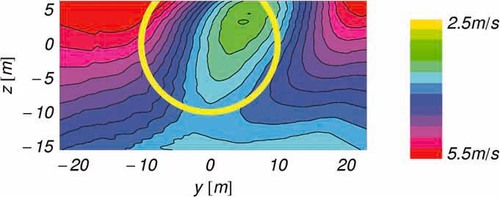
Two-dimensional 10-min average ulos in the nacelle frame of reference. The incomplete circle represents the projection of the rotor in both frames, respectively. Measurement at 80 m downstream (∼4 diameters) on 05.07.2006 from 4:00 to 4:10 a.m.
This misalignment could be explained by combined errors in the lidar and the wind turbine rotor yaw positioning. For instance offsets in pan and tilt, which cannot be fully avoided, are a source for bias. Additionally, there are physical aspects which also contribute. The upward shift can be a consequence of combination of the rotor upward rotor tilt and a slight slope of the terrain. The horizontal misalignment is affected by wrong yaw angle of the turbine with respect to the mean inflow. In effect, no perfect yaw (γ = 0) of the wind turbine can be guaranteed. Therefore an independent combination of both effects is expected. This conclusion is supported by the fact that we were able to observe mean wakes which were more aligned with the rotor axis during other measurement periods. However, for the meandering process what is relevant is the relative wake movement, and this bias should not affect strongly the meandering measurement.
Following the procedure explained in section 3.6, the wind fields were subsequently aligned and averaged over 10 min (see Figure 7). This is expected to eliminate the total turbulent contributions in the wake wind field, thus resulting in a steady wake in the meandering frame of reference. A comparison of this and the mean wake in the nacelle frame of reference is made by extracting the horizontal deficit profiles at the respective wake center and normalizing with respect to mean stream-wise wind speed at hub height. Moreover, the deficit is estimated using the Ainslie model with inflow conditions estimated from the lidar measurements and thrust coefficient (cT = 0.96) obtained from measurements of turbine loading. The comparison of the three deficit profiles is shown in Figure 8. Two consecutive 10-min time series with contrasting behavior are presented, namely the first measured between 3:50 and 4:00 a.m. and the second between 4:00 and 4:10 a.m. The respective estimated wake movement in the horizontal plane is presented in Figure 8(a) and 8(b). In the first case the wind speed deficit profile, resolved in the meandering frame of reference, shows a deficit which is deeper and more slender compared to the resolved in the fixed frame of reference for the measurement (Figure 8(c) and 8(d)). During the first measurement period the turbine changed its yaw position causing a wider wake in the nacelle frame of reference. In contrast, during the next 10 min, the turbine did not change its position, resulting in a similar shape of the wake deficit in both frames of reference (Figure 8(d)). This shows the ability of the tracking and stacking technique to separate meandering, or other large scale effects, from the effects purely due to small scale turbulence.
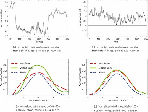
Comparison of 10-min average horizontal profiles of ulos in the meandering and nacelle frame of reference. Fine dashed line represents wake deficit simulated with Ainslie model. Measurement at 80 m downstream (∼4 diameters) on 05.07.2006. Measurement period shown for each of the time series along with the normalization wind speed. Model calculated with estimated Io = 8%.
5.4.2. Turbulence
The 10-min turbulence intensity is obtained following a similar procedure as with the mean wake deficit. The standard deviation of the line-of-sight wind speed is normalized by the mean wind speed at hub height as Ii = σui/ . The resulting two-dimensional field reveals an inhomogeneous structure of the turbulence intensity across the rotor. This is qualitatively in agreement with the expectations from meteorological mast measurements, at least for the fixed frame of reference at hub height, and CFD simulations.10,16
Furthermore, it is assumed that the turbulence intensity in the meandering frame of reference is radially symmetric. Therefore we make an azimuthal averaging; radial profiles with origin at the estimated wake position are extracted at equally spaced angles covering a whole circle. Afterward all of these profiles are averaged and the radial change of the turbulence intensity with respect to the wake center is obtained as in Figure 9.
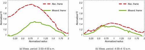
Profiles of 10-min normalized turbulence intensity (Ti) obtained with azimuthal averaging centered at wake center. Data normalized with respect to Io = 8%. Measurement at 80 m downstream (∼4 diameters) on 05.07.2006. Measurement period shown for each of the time series.
The total added turbulence in the fixed frame of reference is assumed as a superposition of wake added turbulence and meandering added turbulence. An insight is given by comparison of the azimuthally averaged profiles resolved in both frames of reference (Figure 9). In the strict sense the azimuthal averaging in the nacelle frame of reference is not correct. A radial symmetry should be expected only when the wake does not meander, for instance in the meandering frame of reference. Therefore, the profile in the nacelle frame of reference in Figure 9(a) is not fully representative of the turbulent field and is used only for qualitative analysis purposes. The higher turbulence values, compared to those in the meandering frame of reference, indicate the existence of additional turbulence. The only source for this added turbulence is the relative movement of the wake when the turbine changed yaw position, and it can be interpreted as an apparent meandering. This conclusion is drawn taking into account that the inflow conditions are very similar for the two time series. Additionally, the effect is not seen for the time series in Figure 9(b) which hardly meanders. Furthermore, a similar qualitative effect should be expected in the fixed frame of reference.
In the meandering frame of reference the measurement shows qualitative and quantitative agreement with comparable results obtained from CFD calculations (cf. e.g. figure 2–40 in Larsen et al.10). The highest turbulence intensity is found in the flow regime where the quasi-steady wake deficit displays large radial gradients. This turbulence decays radially to nondisturbed atmospheric level. This is explained as a combination of the effect of mechanical shear in the wake and break down of tip vortices.10 Eventually, the observed peak will level out far downstream. Furthermore, in the meandering frame of reference the profiles are very similar for both time series. This reveals the ability of the stacking procedure to eliminate great part of the effects of the large scale turbulence as seen in Figure 9(a).
5.4.3. Slanted wake
The steady wake appears to be slanted to the left when looking downstream (see Figure 7, right hand coordinate system with the x coordinate direction pointing downstream). So far, a clear explanation for this has not been found. An influence of the terrain does not seem plausible, since the same effect is seen from opposite wind directions, with fundamental differences in the type of upstream conditions, for instance from inland and from the coast line (Roskilde Fjord). There are, however, two hypotheses that the authors are bearing and trying to cope with.
The effect can be a feature of the wake or it can be just an effect of the measuring and averaging procedure. The first hypothesis could be explained by possible interaction of the intrinsic rotation of the wake and the wind shear. The second hypothesis could be supported by a sort of bias generated by the irregular path of the focus points. As seen in Figure 2 the path it is slanted in the same direction as the wake.
Both effects are difficult to discern from the measured data but two ways are being used to test these possibilities. The slanted shape as a feature of the wake has been checked with detailed CFD simulations of wakes immersed in a vertically sheared flow, and similar phenomena are observed.17 On top of that, Pitot tube measurements of rotor plane flow fields have revealed qualitatively identical characteristics. The second hypothesis is to be coped within new measurements with correction of the driving mechanism of the laser beam.
A direct consequence of the slanted observation is that the correlation coefficient (ρ) should be retained in the bivariate Gaussian function to be fitted during the wake tracking procedure (see equation 2). However, tests show low effect in the relative position prediction with the more elaborated function. Hence, the effect of the slanted wake is expected to be negligible if the interest is in obtaining the relative wake position in time.
6. CONCLUSIONS
Full-scale measurements have been performed in the wake of a middle sized wind turbine (95 kW) by means of lidar. The first part of the paper5 shows the new measurement technique and the analysis of measurements with a one dimensional scanning strategy. This part of the paper deals with the development of analysis methods for the two-dimensional scanning technique. The aim was the quantification of the so called wake meandering as well as the quasi-steady wake deficit and the wake turbulence. The new methods have been applied to different measurement data sets, and here we show in detail analysis of two time series measured under stable atmospheric stratification. The large scale dynamics of the wake could be captured with the created methods. The results reveal a high potential of these measurement and analysis techniques for the recording and understanding of full-scale wind turbine wakes.
The wind field at a particular downstream position can be resolved in a quasi-instantaneous time frame. Based on this, a complete methodology for wake tracking, based on two-dimensional lidar measurements, has been developed and tested. This, has proved to be relatively robust and enables observation of wake dynamics and wake steady characteristics in the fixed and meandering frames of reference.
The measurements were first used to test the Dynamic Wake Meandering (DWM) model when using a moving average window equivalent to two rotor diameters. For the analyzed time series, the model prediction of wake position downstream is very satisfactory. This complements the results of one dimensional measurements already presented in the first part of this paper. The maximum cross-correlation of measured meandering and predicted meandering with the DWM is relatively high, at least for the stable atmospheric conditions evaluated. Moreover, the measurement of the wake in the meandering frame of reference is significant; under wake circumstances, wind turbines observe a more pronounced wind speed deficit moving in front of the rotor compared to that resolved from fixed frame measurements. This is highly relevant for loading simulation.
Furthermore, the obtained qualitative and quantitative information of the organized wake flow structure is also useful for validation of models used in wind farm energy yield assessment. As example a comparison with the Ainslie model has been made. However for generalization purposes thorough statistical analysis has to be performed over different operational conditions.
With these measurements it was possible to observe an apparent effect of vertical wind shear on wake development. Hypothetically the slightly rotating wake is slanted downstream toward one side losing symmetry relatively fast. This finding motivated the investigation through simulation with a CFD model, which has shown the complex interaction of the rotating wake and the shear. However, this is not definitive, since an influence of the scanning strategy cannot be discarded, and further investigation of this phenomenon is being performed.
More measurements have to be analyzed, in particular under less stable atmospheric conditions where stronger meandering is expected. In this way the robustness of the analysis method can be studied and further validation of the basic meandering conjecture can be performed. In this respect the authors are currently preparing further measurement campaigns on wind turbines of different size and with different lidar systems.
Acknowledgements
This research was performed during a research internship at Risø National Laboratory of the corresponding author, and we would like to thank Risø for facilitating this exchange promoted in the framework of the European Academy of Wind Energy (EAWE). The analysis were supported partially by national and European funds through the following projects: ‘RAVE-LIDAR—Development of LIDAR technologies for the German offshore test field’ of The German Federal Environment Ministry (BMU) (Contract No 0327642); Simulation package for generation of wind loads to aeroelastic simulations' of the Danish Energy Agency (Contract No. 33032-0085) and EU project ‘TOPFARM—Next Generation Design Tool for Optimization of Wind Farm Topology and Operation’ (Contract TREN07/FP6EN/S07.73680/038641).


