Developing points-based risk-scoring systems in the presence of competing risks
Abstract
Predicting the occurrence of an adverse event over time is an important issue in clinical medicine. Clinical prediction models and associated points-based risk-scoring systems are popular statistical methods for summarizing the relationship between a multivariable set of patient risk factors and the risk of the occurrence of an adverse event. Points-based risk-scoring systems are popular amongst physicians as they permit a rapid assessment of patient risk without the use of computers or other electronic devices. The use of such points-based risk-scoring systems facilitates evidence-based clinical decision making. There is a growing interest in cause-specific mortality and in non-fatal outcomes. However, when considering these types of outcomes, one must account for competing risks whose occurrence precludes the occurrence of the event of interest. We describe how points-based risk-scoring systems can be developed in the presence of competing events. We illustrate the application of these methods by developing risk-scoring systems for predicting cardiovascular mortality in patients hospitalized with acute myocardial infarction. Code in the R statistical programming language is provided for the implementation of the described methods. © 2016 The Authors. Statistics in Medicine published by John Wiley & Sons Ltd.
1 Introduction
Predicting the occurrence of an adverse event or outcome over time is an important issue in clinical medicine, health services research, and in population and public health. Estimating the incidence of adverse events over time provides clinicians, patients, and policy-makers with important evidence necessary for medical decision making and for making informed policy decisions. Clinical prediction models and associated points-based risk-scoring systems are popular statistical methods for describing the relationship between a multivariable set of patient risk factors and the risk of the occurrence of an adverse event. Popular clinical prediction models and risk-scoring systems in cardiovascular medicine include the Framingham Risk Scores, the EFFECT Heart Failure mortality prediction model, the GRACE risk score, the GUSTO model, and the TIMI risk score 1-9. The Framingham Risk Scores, of which new ones continue to be developed and used, are amongst the oldest, and arguably the most famous, of the existing points-based risk-scoring systems.
While some clinical prediction models focus on predicting the risk of all-cause mortality, there is a growing interest in predicting the risk of the occurrence of outcomes apart from all-cause mortality. Other outcomes of interest include mortality due to cardiovascular causes, hospital readmission or visits to the Emergency Department of hospitals, and incident diagnoses of specific diseases. In patients who have received implantable cardioverter defibrillators (ICD), the incidence of shock or appropriate therapy are outcomes of clinical importance. An important issue when considering outcomes other than all-cause mortality is the existence of competing risks, that is, events whose occurrence precludes the occurrence of the event of interest. When predicting outcomes such as incident cardiovascular disease or Alzheimer's disease over long periods of time (e.g. 30 or more years), competing risks require careful consideration, as the risk of dying from non-disease related causes increases over the duration of follow-up 10-12 and those subjects having this event would no longer be at risk of a disease-related event 13, 14. In the settings described above, deaths from non-cardiovascular disease (when predicting the incidence of cardiovascular disease) or deaths from any cause (when predicting the incidence of Alzheimer's disease) are competing risks. As the competing risk of mortality is more common in high risk populations with long duration of follow-up, their effect may be more pronounced in older, sicker, or more frail longitudinal cohorts than in younger or healthier cohorts.
Conventional statistical methods for the analysis of survival (or time-to-event or event history) data assume that competing risks are absent. Ignoring the presence of competing risks can result in incorrect estimates of the incidence of the event of interest, as well as incorrect estimates of the magnitude of the association between patient characteristics and patient prognosis. For example, estimation of incidence in the presence of competing risks will generally be biased upwards if the competing events are ignored 13-18. If the competing events are independent, then the quantity being estimated is different than the cumulative incidence with competing risks and may not be relevant to clinical decision making. As noted by Pepe and Mori, under independence, the Kaplan–Meier estimator may be interpreted as the probability of the occurrence of the event of interest by time t if the risk of the competing event could be removed 19. In the cardiovascular example, if death from cardiovascular causes and death from other causes are independent, one is estimating incidence (assuming independent competing risks) of cardiovascular death in a population where no one dies from other causes, which may be less relevant than the incidence in a realistic population where death from other causes occurs. Even if such a quantity were clinically relevant, Tsiatis demonstrated that one cannot formally verify whether the competing events are independent of one another 20.
In the absence of competing events, there is a direct relationship between the regression coefficients from a Cox proportional hazards regression model and the relative incidence of the event of interest:
 , where S(t) denotes the survival function for an individual with covariate vector Z, S0(t) denotes the baseline survival function for an individual whose covariates are equal to zero, and β denotes the vector of regression coefficients from the Cox regression model 14. However, in the presence of competing risks, this direct relationship no longer holds if one treats the competing events as censorings. Regardless whether the competing events are independent, the relative effect of a covariate on the cause specific hazard function which censors competing events generally differs from its effect on the cumulative incidence of the event of interest in the presence of competing risks.
Given the increasing interest and focus on outcomes other than all-cause mortality, on predicting the occurrence of specific diseases (e.g. Alzheimer's disease or cardiovascular disease) in high risk populations over long durations, and the importance of providing clinicians, patients and policy-makers with accurate estimates of patient prognosis, our objective is to describe methods for developing simple points-based risk-scoring systems based on the incidence of outcomes in the presence of competing risks. We would like to draw the reader's attention to the fact that our focus is on incidence, which is useful in predictions and prognosis, rather than on cause-specific hazard functions, which are helpful in understanding etiology 13.
The paper is structured as follows. In Section 2, we briefly review statistical methods for survival analysis in the presence of competing risks. We then modify previously described methods for developing clinical prediction models and points-based risk-scoring systems for outcomes in the presence of competing risks. In Section 3, we illustrate the application of these methods in a sample of subjects discharged from hospital with a diagnosis of acute myocardial infarction (AMI). We develop a clinical prediction model and derive a points-based risk-scoring system for predicting cardiovascular mortality in this population of patients. Finally, in Section 4, we summarize our findings and place them in the context of the existing literature. Throughout the paper, we illustrate the development of these risk-scoring systems using the R statistical programming language.
2 Statistical methods for survival data in the presence of competing risks
In this section, we briefly review statistical methods for survival analysis in the presence of competing risks. We then describe how previously described methods for developing points-based risk-scoring systems can be modified to allow one to address the presence of competing risks.
2.1 Review of survival analysis methods in the presence of competing risks
In this section, we provide a brief review of statistical methods for competing risks survival analysis. We do so to provide the reader with the necessary statistical concepts and tools for developing clinical prediction models and points-based risk-scoring systems in the presence of competing risks. Our review is not intended to be exhaustive. For greater background information, the reader is referred to several previously published review articles on this topic 13, 14, 16, 21-23.
2.1.1 Notation and definitions
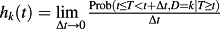
In general survival analysis, in which competing risks are absent, for the ith subject, there is an event time ti and a censoring time ci. The observed survival time for each subject is denoted by xi = min(ti, ci). The censoring indicator, δi = I(ti ≤ ci), denotes whether the event was observed to occur for the ith subject, or whether that subject was censored. An important assumption in conventional survival analysis is that of independent or non-informative censoring 24-26. Under this assumption, subjects who are censored at a given point in time can be represented by those subjects who are still at risk for the occurrence of the event at this same point in time.
Treating subjects who experienced a competing event as though they were censored may result in the violation of the assumption of non-informative censoring. For example, if the primary outcome of interest was cardiovascular death, then the assumption of non-informative censoring assumes that subjects who are treated as censored (at a given time) due to non-cardiovascular death can be represented by those subjects who are still alive (event-free) at that time. However, this assumption may often not be warranted. Subjects who experienced the competing event may often have a systematically different prognosis than subjects who remain event-free. In our example, patients who die of non-cardiovascular causes at a given time are likely to be older than subjects who remain event-free. Older age places subjects at an increased risk of death from non-cardiovascular causes as well as of death due to cardiovascular causes. As mentioned previously, even if the competing events are independent, the interpretation of the naïve analysis which censors at the time of competing events may not be relevant to medical decision making and/or policy making, as such analysis refers to a population in which competing risks do not exist. Great care is needed in deciding whether this interpretation is suitable.
In the absence of competing risks, the survival function of the event time T is S(t), describes the distribution of event times: S(t) = Pr(T > t). The distribution function F(t) = 1 − S(t) = Pr(T ≤ t) describes the incidence of the event over the duration of follow-up. The hazard function is defined as
 . The hazard function, which is a function of time, describes the instantaneous rate of the occurrence of the event of interest in subjects who are still at risk of the event. The cumulative hazard function is defined by
 . The survival and hazard functions are related via the cumulative hazard function: S(t) = exp(−H(t)).
In the presence of competing risks, a subject can experience one of a set of different events or outcomes. Let D be a variable denoting the type of event that occurred (e.g. cardiac death vs. non-cardiac death). In the presence of competing risks, there are two different hazard functions of interest: the cause-specific hazard function and the sub-distribution hazard function. The former is defined as
 13, 14. It denotes the instantaneous rate of failure because of the occurrence of the kth event in subjects who are currently event-free. The sub-distribution hazard function, introduced by Fine and Gray, is defined as
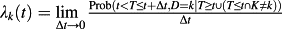 13, 14, 27. It denotes the instantaneous risk of failure from the kth event in subjects who have not yet experienced an event of type k, including those who are currently event-free as well as those who have previously experienced a competing event. One may view the group of individuals experiencing the competing event as ‘immortals’ with respect to events of type k, with their inclusion in the risk set subsequent to the competing event as ‘immortal’ time.
The cumulative incidence function (CIF) for the kth cause is defined as: CIFk(t) = Pr(T ≤ t, D = k). It is the probability of experiencing the kth event prior to time t. The CIF is related to the cause-specific hazard functions:
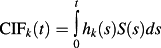 , where S(s) denotes the survival function of the composite outcome of failure due to any cause (which is a function of all the cause-specific hazard functions). As a result, one recognizes that CIFk(t) a function all cause-specific hazards, not just that for the kth cause. On the other hand, similarly to survival data without competing risks, the usual one-to-one relationship exists between CIFk(t) and the subdistribution hazard function λk(t). This property is later shown to be important in the development of points-based risk-scoring systems.
2.1.2 Estimating crude incidence
Estimating the incidence of an event as a function of follow-up time provides important information on the absolute risk of an event. The Kaplan–Meier method is frequently used to estimate the survival function 28. One minus the Kaplan–Meier estimate of the survival function is an estimate of the distribution of event times, which permits one to estimate the cumulative incidence of events over time. However, using the Kaplan–Meier estimate of the survival function to estimate incidence over time in the presence of competing risks can result in biased estimation of incidence 13, 14, 22. In particular, the estimate of incidence is generally biased upwards so that the sum of the Kaplan–Meier estimates of the incidence of each of the individual outcomes will exceed the Kaplan–Meier estimates of the incidence of the composite outcome which is the first time at which any of the competing events occurs. If the events are independent, the Kaplan–Meier estimator estimates the incidence in a hypothetical population where competing events do not exist, which may not be the population of greatest interest for decision and/or policy making 19.
The CIF allows for estimation of the incidence of the occurrence of an event while taking into account the presence of competing events. This allows one to estimate incidence in a population where all competing events must be accounted for in the decision making. The CIF has the desirable property that the sum of the CIFs of the incidence of each of the individual outcomes will equal the CIF of the incidence of the composite outcome consisting of the minimum of all competing event times. Nonparametric estimators for the CIF are well developed, for example, the Aalen–Johansen estimator 29, and are not discussed further in this tutorial.
2.1.3 Hazard function regression
The Cox proportional hazards regression model, whose use is ubiquitous in modern biomedical research, is a regression model that relates the hazard function to a set of covariates. In the absence of competing events, the Cox proportional hazards regression model can be specified as log(h(t)) = log(h0(t)) + βX, where h0(t) denotes the baseline hazard function, X denotes a vector of explanatory variables, and β denotes a vector of regression parameters. An important property of the Cox proportional hazards model in the absence of competing risks is the relation between the regression coefficients and the incidence of the event. The regression coefficients from the above model describe the relative effect of the covariates on the hazard of the occurrence of the outcome. However, the following relationship also holds:
 (where H(t) and S(t) are as described in Section 2.1.1). An important consequence of this relationship is that the relative effect of a given covariate on the hazard of the outcome is equal to the relative effect of that covariate on the logarithm of the survival function. Thus, in the absence of competing risks, making inferences about the effect of a covariate on the hazard function permits one to make similar inferences about the effect of that covariate on prognosis or survival.
In the presence of competing risks, two different hazard regression models are available: modeling the cause-specific hazard and modeling the sub-distribution hazard function. These model the effect of covariates on the cause-specific hazard function and the sub-distribution hazard function, respectively. Lau et al. suggest that cause-specific hazard models are ‘better suited for studying the etiology of diseases, where the [sub-distribution hazard model] has use in predicting an individual's risk’ 13 (p. 245). This view is echoed by Koller et al., who suggested that subdistribution hazard-based methods are preferable when the focus is on estimating actual risks and prognosis 30, as there does not exist a simple one-to-one relationship between the cause-specific hazard and the cumulative incidence for an event of interest. Furthermore, we would note that if one is interested in the overall impact of covariates on the incidence of the outcome of interest, even when predictions of incidence are not of direct interest, then the subdistribution hazard may be of greater interest. We would also note that in the above two references, the term prediction is apparently used to mean predicting the absolute probability of the occurrence of the event of interest. These arguments suggests sub-distribution hazards models should be employed for developing clinical prediction models and risk-scoring systems for time-to-event outcomes in the presence of competing risks. While our focus is on the use of the sub-distribution hazard model, we will also describe briefly how cause-specific hazard functions for the different events of interest can be combined to estimate the cumulative incidence function of a specific event.
Fine and Gray introduced the proportional hazards model for the subdistribution of a competing risk 27: log(λk(t)) = log(λ0,k(t)) + βX, where β denotes the vector of regression coefficients that describe the effect of the covariates on the baseline subdistribution hazard function for the kth event (λ0,t(t)). While this model is frequently referred to as a subdistribution hazard model, it has also been described as a CIF regression model. The reason for this is that the subdistribution hazard function and the CIF are linked through the following formula:
 31.The latter name makes explicit the link between the subdistribution hazard and the effect on the incidence of an event in the presence of competing events. That is, one may directly predict the cumulative incidence for an event of interest using the usual relationship between the hazard and the incidence function under the proportional hazards model.
2.1.4 Statistical software for competing risks analyses
Statistical methods for the analysis of competing risks survival data have been implemented in many popular statistical software packages. In the case study below, we illustrate the application of our methods using the R (version 3.0.2) statistical programming language, and the cmprsk (version 2.2-6) package in particular. In the cmprsk package, one can use the cuminc function to estimate cumulative incidence functions, the crr function to fit subdistribution hazard regression models, and the predict.crr function to estimate the baseline cumulative incidence function from an underlying subdistribution hazard model.
In SAS, PROC PHREG permits estimation of subdistribution hazard models (SAS/STAT version 13.1), while the %CIF macro permits estimation of cumulative incidence functions. In Stata, the stcrreg function permits estimation of subdistribution hazard regression models.
If all subjects had the same duration of follow-up (e.g. five years) and no subjects were lost to follow-up, then one could fit the Fine–Gray model using standard statistical software for fitting the conventional Cox regression model. This can be achieved by recoding competing events as being right censored at five years (so-called censoring complete data). Furthermore, one could also obtain valid nonparametric estimates of the CIF using standard functions for estimating the Kaplan–Meier functions using this coding of the data. Similarly, one could also use standard methods for assessing goodness-of-fit and model performance for the Cox model with this coding of the data. The censoring complete approach generalizes to the case where the independent censoring time is observed on all subjects, as occurs when censoring only occurs because of administrative loss to follow-up at the end of the study. In this case, competing events would be censored at the administrative follow-up time, which might vary across subjects.
2.2 Developing points-based scoring systems in the presence of competing risks
We describe two different frameworks for developing points-based risk-scoring systems in the presence of competing risks. The first is based on the framework used for developing the Framingham Risk Scores and permits the incorporation of both continuous and categorical risk factors. The second is a modification of a framework for use when all of the risk factors are categorical variables 32.
2.2.1 Age-standardized points scoring system using the Framingham framework
In this section, we describe the development of a points-based risk-scoring system in which the points associated with each level of each risk factor are defined relative to the points associated with an increase in a specified continuous variable. This framework reflects the Framingham Risk Score for predicting hard coronary heart disease, in which the points associated with each level of each risk factor are relative to the points associated with a ten-year increase in age. While it is not required that age be included in every risk-scoring system, the incidence of many adverse outcomes increases with increasing age. In the rest of this section, we assume that age is included in the risk-scoring system and that the effects of other risk factors are standardized relative to the effect of age. However, in specific contexts, investigators may choose to standardize the effects of other risk factors relative to a different continuous variable that is part of the risk-scoring system.
Sullivan et al. described a process for developing points-based risk-scoring systems, using the Framingham Risk Score for predicting hard coronary heart disease (i.e. AMI or coronary death) as an example 33. We describe a modification of this approach for use in the presence of competing risk. We refer the interested reader to Sullivan et al.'s detailed tutorial for additional background information and details. For the sake of consistency, the numeric labeling of our steps reflects those of Sullivan et al. Furthermore, we develop a risk score for the k-th event type.
- Step 1 The subdistribution hazard of the event of interest is regressed on the set of risk factors and predictors of the outcome of interest. One of the predictor variables is age, which can be represented as either a continuous variable or a categorical variable. The remaining variables can be either continuous or categorical variables. The regression coefficient (beta coefficient or log-hazards ratio) for each predictor variable is estimated.
- Step 2 While the underlying subdistribution hazard model can incorporate both continuous and categorical covariates, the point scoring system is organized around categories. Thus, clinically meaningful categories of each of the continuous variables must be determined.
- Step 3 The generation of a points-based risk-scoring system requires that one identify a category for each risk factor to serve as the reference level or base category. This reference level or base category will be assigned zero points in the points scoring system. The midpoint of each category that was derived from a continuous variable is then determined. The use of mid-points for each category allows one to determine the distance between each category of the risk factor and the reference level of that category. For determining the midpoint of the lowest category, one may elect to use the first percentile, rather than the minimum value of the variable. Similarly, for determining the midpoint of the highest category, one may elect to use the 99th percentile, rather than the maximum value of that variable. For variables with a small proportion of extreme outliers, such an approach may result in more sensible midpoints for the extreme categories.
- Step 4 Using the estimated regression coefficients from the subdistribution hazard model, determine how far each risk factor category is from the reference category for that risk factor in regression units.
- Step 5 One needs to define the constant B that denotes the number of regression units that reflect one point in the final points-based scoring system. We will follow the convention of the Framingham Risk Scores, in which B denotes the increase in risk associated with a five-year increase in age. Thus, if age is measured in years, B would be set equal to five times the regression coefficient for age in the subdistribution hazard model (estimated in Step 1).
- Step 6 One then calculates the number of points associated with each category of each risk factor. The number of points associated with a given category is defined to be the distance of that category from the reference category for that risk factor (calculated in Step 4) divided by B (defined in Step 5).
- Step 7
One then determines the points total associated with each risk profile (each possible combination) of the different risk categories. This is done by summing up the points associated with each of the risk categories comprising that risk profile. The final step is to determine the incidence of the outcome within a specified duration of time that is associated with each of the possible values of the risk-scoring system. This uses the following sub-steps:
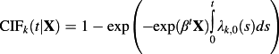
- The cumulative incidence function for a given covariate vector X is equal to
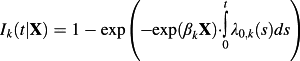 , where λ0,k(t) denotes the baseline subdistribution hazard function for the kth event type: the subdistribution hazard function for the kth event type for a subject's whose covariates are equal to zero 31.
 - From the estimated subdistribution hazard model obtained in Step 1, one can obtain a Breslow-type estimate of the underlying subdistribution hazard function for a reference subject. For a given duration of follow-up, t0, a numeric estimate of the intergral
 can be obtained. 1 − exp(Λ0,k) is the baseline Cumulative Incidence Function (i.e. the CIF for a subject whose covariates are all equal to zero) for the kth event type.
 - A points-scoring system seeks to simplify the application of the prediction model by approximating
 by the sum of the points associated with the given risk factor profile multiplied by the constant B. Thus, in the formula described above in sub-step (a), one replaces βkX by a modification of the sum of the points associated with the given risk factor profile multiplied by the constant B. The modification is necessary because each category that was based on an underlying continuous variable (e.g. age) was represented by the distance (in regression units) from the reference level for that category. Thus, the sum of the points score needs to be modified by adding back the numeric value associated with the reference level (e.g. the mid-point) multiplied by the regression coefficient for the underlying continuous predictor variable. This permits estimation of the incidence of the outcome of interest for each value of the sum of the points.
- The cumulative incidence function for a given covariate vector X is equal to
2.2.2 Regression coefficient-based approach in settings with only categorical risk factors
- Step 1 A Fine–Gray subdistribution hazard model is used to model the subdistribution hazard of the event of interest.
- Step 2 Estimated regression coefficients are then multiplied by 10 and rounded to the nearest integer. The rationale for using the estimated regression coefficients rather than the estimated hazard ratios is that the hazard model is linear in the coefficients, with a one unit change in the covariate having an additive effect on the log-hazard ratio equal to the regression coefficient 32. The resultant integer represents the component of the score for the presence of the given risk factor. Reference levels of the categorical variable are assigned a score of zero. In settings in which some of the predictor variables or risk factors are continuous, the continuous risk factors would need to be categorized into clinically meaningful categorical variables. The requirement that all of the risk factors be categorical is necessary because of the assignment of points to each level of the risk factor, with zero points being assigned to the reference level. The reference level is the category that confers the least risk when the risk has more than two levels.
Once the risk score has been developed and the total value of the points-based risk-scoring system has been determined for each subject, subjects can be divided into appropriately sized risk strata. There is no universally agreed upon number of strata that are appropriate. Indeed, the choice of the number of strata is likely to be influenced by the clinical and policy context. However, it appears that five risk strata are used in many applications and clinical settings. In our case study, we will consider using five risk strata. This can be done by dividing subjects into five equally sized groups using the quintiles of the estimated risk score. The incidence of the outcome of interest can then be estimated within each of the risk strata using the empirical CIF.
3 Case study
3.1 Data sources
The Enhanced Feedback for Effective Cardiac Treatment (EFFECT) Study was a study designed to assess the effect of public reporting of hospital performance on the quality of care provided to patients with cardiovascular disease in Ontario, Canada 36. During the study, detailed clinical data on patients hospitalized with acute myocardial infarction (AMI or heart attack) between April 1, 1999 and March 31, 2001 (Phase 1) and between April 1, 2004 and March 31, 2005 (Phase 2) at 103 hospitals in Ontario, Canada were obtained by retrospective chart review. Data on patient demographics, vital signs and physical examination at presentation, medical history, and results of laboratory tests were collected by trained cardiovascular nurse abstractors. The initial sample consisted of 15 569 subjects. Four hundred five (2.6%) subjects with missing data on continuous baseline covariates necessary to estimate the risk score were excluded from the current case study, leaving 15 164 patients for analysis (10 063 patients in Phase 1 and 5101 patients in Phase 2).
For the current study, we restricted our analyses to subjects who were discharged alive from the index hospitalization recorded in the EFFECT study. Subjects were then linked deterministically, using an encoded version of the patient's Ontario health insurance number to the Vital Statistics database maintained by the Ontario Office of the Registrar General. The Vital Statistics database contains information on date of death and cause of death (based on ICD-9 codes) for residents of Ontario. Each subject was followed for five years from the date of hospital discharge for the occurrence of death. For those subjects who died within five years of discharge, the cause of death was noted in the Vital Statistics database. For the purposes of these analyses, cause of death was categorized as cardiovascular vs. non-cardiovascular causes of death. Four thousand two hundred and seventy-six (28%) patients died during the five years of follow-up. Of these, 2518 (59%) died of cardiovascular causes, while 1758 (41%) died of non-cardiovascular causes.
The following predictor variables were selected a priori for inclusion in regression models predicting the occurrence of cardiovascular death: age, heart rate, systolic blood pressure, initial serum creatinine, history of AMI, history of congestive heart failure, ST-depression myocardial infarction, elevated cardiac enzymes, and in-hospital percutaneous coronary intervention. The first four variables are continuous variables, while the last five are dichotomous risk factors. These nine variables were selected because they are components of the GRACE risk score for predicting mortality in patients with acute coronary syndromes 5.
While the four continuous covariates were incorporated as continuous variables in the subdistribution hazard model, the points scoring system is organized around categories. Thus, for the purposes of presentation, an a priori decision was made to categorize the four continuous covariates as follows: Age (in years): <65, 65–74, ≥75; Systolic blood pressure (in mm Hg): <90, 90–109, 110–129, ≥130; Heart rate (in beats per minute): <60, 60–99, 100–119, ≥120; and Creatinine: < 90 µmol/L, 90–179 µmol/L, ≥ 180 µmol/L (in SI units) (equivalent to <1.02 mg/dL, 1.02 – 2.02 mg/dL, ≥ 2.02 mg/dL in non-SI units used in the United States). The categories were defined prior to data analysis, using clinically meaningful categories determined by a clinician co-author (DSL).
3.2 Descriptive statistical analyses
Descriptive statistics for patients in the study sample are reported in Table 1. Continuous variables were summarized using medians and the 25th and 75th percentiles, while dichotomous variables were summarized using frequencies and percentages.
| Variable | N (%) or median (IQR) |
|---|---|
| Age (years) | 69 (57–78) |
| Age < 65 years | 6157 (40.6%) |
| Age 65–74 years | 3682 (24.3%) |
| Age ≥ 75 years | 5325 (35.1%) |
| Heart rate at admission (beats per minute) | 80 (68–97) |
| Heart rate < 60 | 1755 (11.6%) |
| Heart rate 60 – 99 | 9931 (65.5%) |
| Heart rate 100 – 119 | 2213 (14.6%) |
| Heart rate ≥ 120 | 1265 (8.3%) |
| Systolic blood pressure at admission (mmHg) | 146 (126–168) |
| Systolic blood pressure < 90 | 354 (2.3%) |
| Systolic blood pressure 90 – 109 | 1205 (8.0%) |
| Systolic blood pressure 110 – 129 | 2730 (18.0%) |
| Systolic blood pressure ≥ 130 | 10 875 (71.7%) |
| Previous AMI | 3574 (23.6%) |
| Previous congestive heart failure | 734 (4.8%) |
| Creatinine (µmol/L)* | 92 (78–113) |
| Creatinine < 90 | 6780 (44.7%) |
| Creatinine 90 – 179 | 7518 (49.6%) |
| Creatinine ≥ 180 | 866 (5.7%) |
| Elevated cardiac enzymes | 14 472 (95.4%) |
| ST elevation AMI | 6625 (43.7%) |
| Percutaneous coronary intervention in hospital | 596 (3.9%) |
- * To convert creatinine to US units (mg/dL), divide by 88.4.
Cumulative incidence functions describing the cumulative incidence of cardiovascular and non-cardiovascular death in the overall sample are described in Figure 1, along with the incidence of the composite outcome of all-cause mortality. The cumulative incidence of all-cause mortality is equal to the sum of cumulative incidences of the two cause-specific mortalities. The cumulative incidence of cardiovascular death exceeded that of non-cardiovascular death at each point in time. As suggested by Pepe and Mori, a figure similar to Figure 1 should be presented when estimating cumulative incidence in the presence of competing risk 19.

3.3 Age-standardized points scoring system
R code and output describing the development of this points-based risk-scoring system are described in Section A of the Supporting Information (once the regression models have been fit, the calculation of the points associated with each patient profile can also be done using commonly available software such as Microsoft Excel ™). The first step was to use a Fine–Gray competing risk regression model to regress the subdistribution hazard of cardiovascular death on four continuous variables: age, systolic blood pressure at admission, heart rate at admission, initial creatinine after admission, and five binary variables: history of AMI, history of congestive heart failure, ST-depression myocardial infarction, elevated cardiac enzymes, and no in-hospital percutaneous coronary intervention. The estimated regression coefficients, sub-distribution hazard ratios, estimated 95% confidence intervals, and statistical significance of the estimated regression coefficients are reported in Table 2.
| Variable | Log-hazard ratio (β) | Sub-distribution hazard ratio | 95% CI for hazard ratio | P-value |
|---|---|---|---|---|
| Age (per year increase in age) | 0.0644 | 1.07 | (1.06,1.07) | <0.0001 |
| Heart rate (per beat per minute) | 0.0074 | 1.01 | (1.01,1.01) | <0.0001 |
| Systolic blood pressure (per mmHg) | −0.0045 | 1.00 | (0.99,1.00) | <0.0001 |
| Previous myocardial infarction | 0.4754 | 1.61 | (1.48,1.75) | <0.0001 |
| Previous congestive heart failure | 0.49 | 1.63 | (1.44,1.86) | <0.0001 |
| Creatinine (per µmol/L)* | 0.0021 | 1.00 | (1.00,1.00) | <0.0001 |
| Elevated cardiac enzymes | 0.131 | 1.14 | (0.93,1.40) | 0.2200 |
| ST-elevation AMI | −0.174 | 0.84 | (0.77,0.92) | 0.00019 |
| No PCI during hospital admission † | 0.5172 | 1.68 | (1.16,2.42) | 0.0057 |
- * To convert creatinine to US units (mg/dL), divide by 88.4.
- † PCI = percutaneous coronary intervention.
The discrimination of the subdistribution hazard model was assessed using Wolber's concordance index for prognostic models with competing risks 37. The apparent discrimination for the occurrence of cardiac death within 1, 2, 3, 4, and 5 years were equal to 0.701, 0.690, 0.689, 0.699, and 0.696, respectively. Estimates of the concordance index at 1, 2, 3, 4, and 5 years using bootstrap cross-validation with 1000 bootstrap samples were 0.700, 0.690, 0.689, 0.699, and 0.696, respectively. The calibration of the model was assessed graphically by comparing the predicted probability of cardiac death within five years to the observed probability of cardiac death within five years across the 10 deciles of predicted risk (Figure 2) 31. Overall, the model displayed good calibration, with a modest degree of under-prediction in subjects in the 8th and 9th deciles of predicted risk.

The four continuous predictor variables (age, systolic blood pressure, heart rate, and creatinine) were modeled as continuous variables in the subdistribution hazard model described above. However, the points scoring system is organized around categories. The second step in the process is to categorize these variables using the categorization described previously.
The third step was to determine the midpoint of each category derived from a continuous variable and define the reference level for each risk factor.
In the fourth step, we determined how far each risk factor category is from the reference level for that risk factor in regression units.
In the fifth step, we developed a point scoring system in which the points associated with each risk factor category were relative to the incremental effect of a five-year increase in age on the subdistribution hazard of cardiovascular death. Thus, B (the constant) is equal to five times the regression coefficient for age from the subdistribution hazard model estimated in Step 1.
The sixth step entailed determining the points associated with each level of each risk factor in age-standardized units. The points assigned due to the presence or absence of each risk factor are reported in Table 3. The reference patient, with a score of zero is a patient aged 21–25 years old, with systolic blood pressure less than 90 mmHg, heart rate on admission of less than 60 bpm, creatinine of less than 90, with no previous AMI, no previous congestive heart failure, no elevated cardiac enzymes, no ST-elevation myocardial infarction, and who received PCI during the hospital admission. Thus, having a history of previous congestive heart failure results in the assignment of two points towards the total points score. Similarly, having a heart rate of 120 beats per minute or higher results in the assignment of two points towards the total points score. The minimum theoretical score is −2 while the maximum theoretical score (assuming a maximum age of 100 years) is 23.
| Variable | Points |
|---|---|
| Age (per increase of five years over age 21–25) | 1 |
| Heart rate: <60 | 0 |
| Heart rate: 60–99 bpm | 1 |
| Heart rate: 100–119 bpm | 1 |
| Heart rate: ≥120 bpm | 2 |
| Systolic BP: 0–89 mm Hg | 0 |
| Systolic BP: 90–109 mm Hg | 0 |
| Systolic BP: 110–129 mm Hg | −1 |
| Systolic BP: ≥130 mm Hg | −1 |
| Previous myocardial infarction | 1 |
| Previous congestive heart failure | 2 |
| Creatinine: <90 µmol/L | 0 |
| Creatinine: 90–179 µmol/L | 0 |
| Creatinine: ≥180 µmol/L | 1 |
| Elevated cardiac enzymes | 0 |
| ST-elevation AMI | −1 |
| No PCI during hospital admission | 2 |
The seventh step was to determine the total points assigned for each subject in the sample. The minimum and maximum observed scores in the sample were 1 and 22 respectively. The median score was 11, while the 25th and 75th percentiles were equal to 8 and 13, respectively.
We now determine the baseline cumulative incidence function for a subject whose covariate values are equal to zero. This will be used to determine the incidence of cardiac death associated with any value of the risk score. We extract the estimated incidence of cardiac death at 1, 2, 3, 4, and 5 years subsequent to hospital discharge.
Finally, we determine the incidence of cardiac death at 1, 2, 3, 4, and 5 years for each of the possible values of the risk score. To do so, we multiply the value of the risk score by B and add back the value of the midpoint of the reference level of each continuous risk factor multiplied by the regression coefficient associated with that continuous variable. Thus, a patient hospitalized with AMI with a risk score of 10, would have a 0.036 probability of death due to cardiovascular causes within one year of hospital discharge and a 0.051 probability of death due to cardiovascular causes within two years of hospital discharge. The association between each possible value of the risk score and the one-, two-, three-, four-, and five-year incidence of cardiac death are described in Figure 3.

Subjects in the study sample were divided into five risk strata using the quintiles of the estimated age-standardized risk score. Cumulative Incidence Functions for cardiovascular death were estimated within each of the five risk strata (left panel of Figure 4). Stratification on the five risk strata defined by the quintiles of the age-standardized points score permitted effective risk stratification of AMI patients. There existed a strong gradation in the incidence of cardiovascular death across the five strata.

Latouche et al. suggested that competing risks analyses should report all of the cause-specific cumulative incidence functions 38. To do so, within each of the five strata defined by the quintiles of the risk score for cardiovascular death, we estimated the CIFs for non-cardiovascular death. These are reported in the right panel of Figure 4. In each of the five risk strata, the cumulative incidence of non-cardiovascular death did not exceed the cumulative incidence of cardiovascular death. In the stratum with the lowest risk of cardiovascular death, the risk of non-cardiovascular death was approximately equal to the risk of cardiovascular death. However, the difference between the two cause-specific CIFs increased across the five strata of cardiovascular death. In the highest-risk stratum, the cumulative incidence of cardiovascular death was almost twice that of non-cardiovascular death. The R code for producing this figure is provided in the Supporting Information.
To examine loss of predictive accuracy because of the use of the age-based points scoring system, we regressed the incidence of cardiac death on a single variable denoting each subject's score. The discrimination and calibration of this model were examined using methods similar to those described when considering the full subdistribution hazard model. The apparent discrimination for the occurrence of cardiac death within 1, 2, 3, 4, and 5 years were equal to 0.696, 0.679, 0.672, 0.682, and 0.680, respectively. Estimates of the concordance index at 1, 2, 3, 4, and 5 years using bootstrap cross-validation with 1000 bootstrap samples were 0.695, 0.678, 0.672, 0.681, and 0.678, respectively. The decrease in discrimination between this model and the full subdistribution hazard model was minimal. The calibration of this model is described in Figure 2. There was no meaningful difference in calibration between this model and that of the full subdistribution hazard model.
3.4 Categorical variable-based points scoring system
In the previous section, we described the development of a points-based risk-scoring system based on the process of age-standardization of regression coefficients, as used in the development of the Framingham Risk Scores. In this section, we illustrate the application of the second approach for developing a points-based risk-scoring system that requires that all of the risk factors be categorical variables. A Fine–Gray hazard model was used to model the subdistribution hazard of cardiovascular death as a function of the nine covariates described above. Because this procedure is applicable to settings in which the risk factors are categorical, we elected to categorize the continuous risk factors so that the procedure could be applied to the same dataset as was used for the first method. All nine covariates were treated as categorical variables using the previously described categorizations. R code and output for developing this points-based risk-scoring system are described in Section B of the Supporting Information.
The regression coefficients for the Fine–Gray subdistribution hazard model fit to the overall sample are reported in Table 4. In the right-most column of the table are the points associated with the presence of a given level of a risk factor (with the reference level being assigned zero points) (as described above, the points were determined by multiplying the regression coefficient by 10 and rounding to the nearest integer). Advanced age (≥75 years old) conferred the largest number of points (17). The theoretical minimum and maximum sum of the points were −12 and 45, respectively. The observed scores in the EFFECT-AMI sample ranged from −11 to 45. The median score was 13, while the 25th and 75th percentiles were 4 and 23, respectively.
| Variable | Log-hazard ratio (β) | Hazard ratio | 95% CI for hazard ratio | P-value | Points |
|---|---|---|---|---|---|
| Age 65–74 | 0.9280 | 2.53 | (2.19,2.93) | <0.0001 | 9 |
| Age ≥ 75 | 1.7191 | 5.58 | (4.90,6.36) | <0.0001 | 17 |
| Heart rate 60–99 | 0.4611 | 1.59 | (1.35,1.86) | <0.0001 | 5 |
| Heart rate 100–119 | 0.8140 | 2.26 | (1.89,2.69) | <0.0001 | 8 |
| Heart rate ≥ 120 | 0.8542 | 2.35 | (1.95,2.83) | <0.0001 | 9 |
| Systolic BP 90–109 | −0.0425 | 0.96 | (0.73,1.26) | 0.7600 | 0 |
| Systolic BP 110–129 | −0.1591 | 0.85 | (0.66,1.10) | 0.2200 | −2 |
| Systolic BP ≥ 130 | −0.4128 | 0.66 | (0.52,0.85) | 0.0010 | −4 |
| Creatinine 90–179 µmol/L | 0.3983 | 1.49 | (1.36,1.63) | <0.0001 | 4 |
| Creatinine ≥ 180 µmol/L | 0.8733 | 2.39 | (2.08,2.76) | <0.0001 | 9 |
| Previous AMI | 0.4488 | 1.57 | (1.44,1.71) | <0.0001 | 4 |
| Previous heart failure | 0.4980 | 1.65 | (1.45,1.87) | <0.0001 | 5 |
| Elevated cardiac enzymes | 0.1421 | 1.15 | (0.94,1.41) | 0.1700 | 1 |
| ST-elevation AMI | −0.1828 | 0.83 | (0.76,0.91) | <0.0001 | −2 |
| PCI during hospitalization | −0.5914 | 0.55 | (0.38,0.80) | 0.0018 | −6 |
Subjects in the overall sample were divided into five equally sized risk strata using the quintiles of the empirical risk score. The Cumulative Incidence Functions for cardiovascular mortality in each of the risk strata in the overall sample are described in the left panel of Figure 5. There were statistically significant differences in the CIFs across the five risk strata (P < 0.0001). There was a clearly defined gradation in the incidence of cardiovascular death across the five risk strata. The lowest risk stratum comprised subjects with a very low incidence of cardiovascular death during five years of follow-up. In contrast, the highest risk stratum consisted of subjects with a very high incidence of cardiovascular death during five years of follow-up. The five-year incidence of cardiovascular death in the lowest and highest risk strata were 0.024 and 0.410, respectively. Thus, the incidence of cardiovascular death at five years was 17 times greater in the highest risk stratum than in the lowest risk stratum. The corresponding estimates of the CIFs of non-cardiovascular mortality are described in the right panel of Figure 5.

To examine loss of predictive accuracy due to the categorization of variables, we regressed the incidence of cardiac death on a single variable denoting each subject's score. The discrimination and calibration of this model were examined using methods similar to those described above for use with the full subdistribution hazard model considered above. The apparent discrimination for the occurrence of cardiac death within 1, 2, 3, 4, and 5 years were equal to 0.701, 0.707, 0.698, 0.702, and 0.698, respectively. Estimates of the concordance index at 1, 2, 3, 4, and 5 years using bootstrap cross-validation with 1000 bootstrap samples were 0.702, 0.707, 0.700, 0.704, and 0.699, respectively. There was no meaningful difference in discrimination between this approach and that of full subdistribution hazard model.The calibration of this model is described in Figure 2. As with the age-based points scoring system, there was no meaningful change in calibration compared to that of the full subdistribution hazard model.
4 Discussion
Predicting the absolute risk of the event of interest is an important issue in clinical medicine. Accurate estimation of absolute risk permits effective clinical decision making and risk stratification of patients. There is a growing interest in predicting the probability of the occurrence of events other than all-cause mortality. When the focus is on outcomes other than all-cause mortality, the presence of competing events precluding the event of interest should be taken into account. Clinicians are often interested in developing points-based risk-scoring systems that assign points to the presence of different risk factors, and that then quantify patient prognosis associated with different values of the total point score. The Framingham Risk Scores comprise a popular family of points-based risk-scoring systems 2. In this tutorial article, we have described procedures for developing points-based risk-scoring systems in the presence of competing risks.
In the current paper, we described procedures to develop a points-based risk-scoring system in the presence of competing risks, assuming the existence of an underlying prognostic model, namely the Fine and Gray subdistribution hazard regression model. While we have described methods for assessing model performance, we have not discussed issues such as methods for model development. The interested reader is referred to excellent references on methods for developing multivariable regression models 39, 40. General principles for developing multivariable competing risk regression model (e.g. variable selection, identifying the functional form of continuous covariates, determining whether interactions are present) would be similar to those for developing logistic regression models for binary data or Cox proportional hazards models for survival data without competing risks.
It is important to present results for all causes when analyzing the cumulative incidence for different event types with competing risks data 38. Examination of all cause-specific CIFs enables a more complete understanding of the risks of the different outcomes in the study sample. Decision makers need to consider the risks of all events, including non-cardiovascular mortality in treatment planning. Someone with high risk of non-cardiovascular mortality, but with a low risk of cardiovascular mortality may be treated differently than someone with low risk of non-cardiovascular mortality and high risk of cardiovascular mortality. For instance, the latter patient may be an excellent candidate for early cardiovascular revascularization procedures, while the former may not be a suitable candidate for early revascularization. Similarly, depending on further indications, the latter may be a candidate for an ICD, while the former may not be a suitable candidate for ICD implantation. For further examination of this last clinical question, the reader is referred to two different analyses of predictors of the competing risks of appropriate ICD therapy or prior death 41, 42. We examined cause-specific cumulative incidence of each of the causes of death in each of the five risk strata defined by the point-scoring system for cardiovascular death.
A complementary approach, which is beyond the scope of the current paper, would be to develop a separate point-scoring system for non-cardiovascular death in patients hospitalized with AMI. This approach would require development of a second sub-distribution hazard model and knowledge of those variables that increase the incidence of non-cardiovascular mortality in patients hospitalized with AMI. One could then use the two separate point-scoring systems to identify subsets of patients at high risk for cardiovascular death while being at low risk for non-cardiovascular death, and patients at low risk for cardiovascular death while being at high risk for non-cardiovascular death. An advantage to the currently used approach is that the focus was on cardiovascular mortality and the current approach allowed us to examine the incidence of non-cardiovascular mortality in different risk strata for cardiovascular mortality.
Many clinicians find the simplicity of points-based risk-scoring systems appealing, as well as the ease with which they can be used in routine clinical practice. However, we would stress that a points-based risk-scoring system is not necessary for estimating patient prognosis in the presence of competing risks. Instead, one can use the fitted sub-distribution hazard model to estimate directly the incidence of the outcome of interest for any risk factor profile. While such an approach would be difficult to implement by hand or through a simple tabular approach, it can readily be implemented using computers or hand-held electronic devices. In today's environment of mobile computing and web-based risk calculators, some would question the need for developing points-based risk-scoring systems. From a statistical and computing perspective, such points-based risk-scoring systems may seem unnecessarily crude when estimates of incidence can be derived directly from the underlying regression model. As statisticians, we are sympathetic with such an argument. However, this ignores the reality of clinical decision making in fast-paced environments such as the emergency department (ED) or in the clinic 43. Drescher et al., in examining the acceptability of a computerized decision support system in the ED, found that a computerized system was poorly accepted by ED physicians 44. One of the reasons for the poor acceptance was the increased computer time required to enter the necessary information. In contrast, the CHADS2 risk index 45, which is a simple points-based risk-scoring system for assessing the risk of stroke in patients with atrial fibrillation, is widely used by ED physicians 46. An advantage to a simple points-based risk-scoring system, such as CHADS2, is that all the necessary calculations can be made mentally by the clinician without recourse to an electronic device. Such a risk-scoring system can be quickly and easily used to make treatment decisions in a fast-paced environment such as the ED. While points-based risk-scoring systems may have limited utility for research purposes, it appears that they continue to serve a role in supporting clinical decision making, particularly in settings which are subject to time and or resource constraints.
In this tutorial, we focused on risk-scoring systems using the Fine–Gray subdistribution hazard regression model in the presence of competing risks, with the regression coefficients in this model directly related to the magnitude of the effect of the covariate on the CIF. The availability and interpretability of these coefficients lends themselves to creating weights or points associated with the presence of different risk factors. Several authors have described how the CIF can be estimated by estimating cause-specific hazard models for each of the competing events 31, 47, 48. A disadvantage to the approach based on combining cause-specific hazard functions is that it does not result in an estimated regression coefficient summarizing the effect of a given covariate on the CIF. As such, this method does not lend itself to the construction of points-based risk-scoring systems in which weights are assigned for the presence of different risk factors. In comparing the two approaches, Wolbers et al. found that estimates of the incidence of cardiovascular disease in elderly women obtained using a Fine–Gray sub-distribution hazard model were similar to those obtained by combining cause-specific hazard functions 31. We believe that this occurs in many applications and that the choice of which approach to use for points-based risk-scoring systems should be based in large part on convenience and ease of implementation of the scoring system.
There is a growing awareness of the impact of competing risks when developing prognostic models. Wolbers et al. compared the performance of a standard Cox survival model with that of a Fine–Gray model for predicting the incidence of coronary heart disease in older women 31. They found that the standard Cox model overestimated the 10-year risk of coronary heart disease. Using this standard approach, 18% of subjects were classified as being high risk, whereas the Fine–Gray model only classified 8% of subjects as being high risk. They attribute this discrepancy to the increased risk of death due to competing risks in this elderly population. Koller et al. reviewed 50 clinical studies conducted in subjects susceptible to competing risks that were published in high-impact journals and found competing risks issues in 70% of the studies 30. The high prevalence of clinical studies in which competing risks are present suggests that investigators, analysts and readers need to be aware of different statistical methods for addressing research questions in the presence of competing risks. The proposed point-based risk-scoring systems for competing risks data may permit more effective risk stratification and assessing patient prognosis when the focus is on non-fatal outcomes or death because of specific causes.
Acknowledgements
This study was supported by the Institute for Clinical Evaluative Sciences (ICES), which is funded by an annual grant from the Ontario Ministry of Health and Long-Term Care (MOHLTC). The opinions, results, and conclusions reported in this paper are those of the authors and are independent from the funding sources. No endorsement by ICES or the Ontario MOHLTC is intended or should be inferred. This research was supported by an operating grant from the Canadian Institutes of Health Research (CIHR) (MOP 86508). Dr. Austin was supported by Career Investigator awards from the Heart and Stroke Foundation. Dr. Lee is supported by a clinician-scientist award from the Canadian Institutes of Health Research. The Enhanced Feedback for Effective Cardiac Treatment (EFFECT) data used in the study was funded by a CIHR Team Grant in Cardiovascular Outcomes Research. These datasets were linked using unique encoded identifiers and analyzed at the Institute for Clinical Evaluative Sciences (ICES). This study was approved by the institutional review board at Sunnybrook Health Sciences Centre, Toronto, Canada.