Evidence, eminence and extrapolation

1 Introduction

One of the most challenging tasks in medicine is clinical research in children. In the following paper, we look at drug development in the paediatric population. For decades, it has been criticized that most medicines have not been authorized for the use in children. Off-label use based on the individual responsibility of the treating paediatrician is often the only way how children can benefit from medicines that are only authorized for adults 1. This relies on the questionable assumption, that children are small adults. There exist several reasons for such a development: clinical research in children is a sensitive area involving emotional and ethical challenges, methodological challenges, for example, the small numbers of children that can be recruited into trials, and on the other hand increased costs that may not be compensated by economic returns if the treated disease is rare in children. In order to improve the situation, new legal requirements have been created in the USA 2, 3 and in the European Union (EU) 4, 5. Essentially, these require companies to agree a plan for developing a medicine in children with the regulatory authorities before authorization in adults. If studies in children performed according to the agreed plan are submitted and lead to authorization in children, patent exclusivity is prolonged as a reward for the extra effort of the drug developer.

The scope of such a paediatric investigation plan (PIP) may reach from a full programme (including pre-clinical research, pharmacokinetics, pharmacodynamics, dose finding studies and two fully powered pivotal phase III studies) for diseases only existing in childhood at the upper end of the spectrum and, for example, a single (pharmacokinetic) case series in children on the lower end of the spectrum. The latter situation is obviously based on the assumption that data and results from adult patients can be extrapolated to the childhood and only very limited additional data from children are necessary before authorization of the treatment also for children. Such extrapolation is only possible in situations where it may be assumed that children are reasonably similar to adults, which, as a general rule is not acceptable, for example, because of differences related to growth and maturation. In order to give some structure in the decision process whether and to what extent extrapolation from adults to children is appropriate, the Food and Drug Administration (FDA) has developed a paediatric study decision tree based on similarity of disease progression, similarity of response to treatment and similar concentration–response relationships 6.

The European Medicines Agency (EMA) has issued a concept paper on extrapolation 7 that – although referring also to extrapolation in other areas of drug development – has been mainly driven by its Paediatric Committee. Extrapolation in the regulatory context is defined by

Extending information and conclusions available from studies in one or more subgroups of the patient population (source population), or in related conditions or with related medicinal products, to make inferences for another subgroup of the population (target population), or condition or product, thus reducing the need to generate additional information (types of studies, design modifications, number of patients required) to reach conclusions for the target population, or condition or medicinal product.

In the same document, it is stated that the

primary rationale for extrapolation is to avoid unnecessary studies in the target population for ethical reasons, for efficiency, and to allocate resources to areas where studies are the most needed.

There are different ways mentioned on how to reduce the evidence required from the paediatric population(s) dependent on the degree of similarity to the source population (e.g. adults): instead of a full development programme, only a reduced set of studies are required, for example, pharmacokinetic/pharmacodynamic studies only, dose-ranging or dose-titration studies, non-controlled descriptive efficacy and/or safety studies, controlled studies but arbitrary sample size, larger significance level, lower coverage probability of confidence intervals, acceptance of surrogate endpoints for the primary analysis, interpolation (bridging), for example, between age subgroups, modelling prior information from existing data sets (Bayesian models and meta-analytic predictive). Some of these proposals have also been mentioned in the previous EMA guideline on clinical trials in small populations 8.

It is obvious that decisions on the extent of extrapolation possible, for example, from adults to children, are generally not conventional statistical decisions. Often it is even hard to find sufficient data on the control therapy the new treatment has to be compared with in children. Generally, no data at all are available from systematic studies with the new (drug) in children, because we still encounter the argument that paediatric studies are not ethical before the drug has been successfully registered in adults. However, the PIP by European law should be laid down as soon as results from early studies in adults become available, hence, certainly before registration in adults. The rationale behind is that drug developers should provide an early commitment for what they are planning regarding development for children. Often clinical data on the efficacy and safety of the new treatment are very limited even in adults so that decisions will have to be grounded predominantly on expert opinion of experienced specialists in the disease area with corresponding expertise in the paediatric population. Clearly, historical data from different sources and of different relevance will in general play an important role in the expert judgement and decisions. As a matter of fact, decisions under uncertainty have to be taken in this area by experts in collaboration with statisticians. If methodologists refuse to deal with such an environment, the paediatricians will individually decide and apply treatments to children off label without being able to refer to any systematic study results.

In this paper, we will try to structure the extrapolation process. Thereby, we concentrate on softening the burden of evidence in paediatric populations by enlarging the significance level in a paediatric clinical trial. We introduce prior probabilities for non-applicability of extrapolation (‘scepticism’) and priors on the hypotheses to be tested. We show, how single standard frequentist tests with an enlarged significance level correspond to Bayesian decision rules based on certain scepticism and priors. In Section 2, we develop the general framework for α-level adjustment by applying Bayesian arguments. In Section 3, we apply this framework to treatment–control comparisons assuming normally distributed outcome variables. In Section 4, we show as an example, how the FDA decision tree for extrapolation may be roughly embedded in our framework. We close with a short discussion in Section 5. In the Appendix, we show the favourable properties of two-point priors we used in the argumentation.

2 A simple framework for α-level adjustment

Here, H₀ and H₁ indicate the null and alternative hypotheses in, for example, the comparison of the means between an experimental treatment and a control, or in the test of a dose–response relationship.

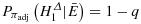
It should be mentioned that criterion (ii) is in contrast to the usual clinical trial approach, where both P(φ = 1|H₁) and P(φ = 1|H₀) are adequately controlled. In our framework, the direct control of the power and the positive predictive value of a significant test result is the crucial condition for comparing different tests. In the conventional testing set-up, the control of the latter value is indirectly aimed at by control of the type I error rate. Thus, our setting could be seen as a compromise between the classical framework and the control of both the positive and the negative predictive value as suggested in 9.

The choice of 1 − β is typically based on economical and ethical arguments, and values of β being equal to 0.1 or 0.2 are traditionally taken in phase III studies. In the following, we will consider two scenarios, where the first scenario will help us to choose a reasonable value also for 1 − γ, which then will hold as a standard, whereas the second scenario will eventually motivate an adjustment of the type I error rate in order to maintain this standard.

2.1 Two scenarios to arrive at the same positive predictive value

2.1.1 The benchmark scenario

To motivate the choice of the positive predictive value 1 − γ, we consider the case that a full study programme is conducted only in the target population, and several early phase studies have been conducted with a positive result including a phase II proof of concept study. With each positive result, the belief in H₁ may have strengthened, and when planning the phase III study, we have arrived at a prior probability for H₁ of 1 − r. We will refer to this scenario as the benchmark scenario. In order to justify this designation, the type I and type II error rates on which depends on are assumed to be the traditional values for phase III studies: α may be set to the one-sided levels 0.025, or even 0.025² (representing the two pivotal studies paradigm), whereas β may be set to, for example, 0.1 or 1 − 0.9²=0.19 (again for the two studies paradigm). Note, P_r(H₁|φ = 1) is given by Bayes's theorem, and the subscript r indicates that this benchmark belief depends on 1 − r. After choosing error rates that represent the common practice in the given setting, let φ_b denote a test that controls exactly these α and β levels.

A crucial parameter in this setting is the value of 1 − r, the regulators belief in H₁. As 1 − r represents the belief before phase III in a standard drug development programme is started, one may argue that enough evidence has been accumulated so that . For the choice of 1 − r, it may be possible to derive an average subjective probability in the Bayesian sense for the truth of H₁. Another possibility is the deduction of 1 − r in a frequentist framework using the law of total probability (see also 9): let φ_III denote a binary function that indicates the success (φ_III=1) or failure (φ_III=0) of a phase III clinical trial. Here, as an example, we consider drug development in oncology. Investigations of the success rates of these phase III trials in oncology claim that approximately 55–60% of these drugs fail 10, 11. Taking this value into account with P(φ_III=1) = 0.40, we have

(1)

by simple algebra it follows

(2)

The value 0.5 in the last equation follows, if αis considered to be negligibly small and if β≈0.2. If the success rate in phase III is higher, the aforementioned derivation will result in an increased prior probability 1 − r > 0.5.

2.1.2 The α-level adjustment scenario

After arriving at a benchmark, two different statistical models have to be considered: one for the source population and one for the target population. In the former model, an alternative hypothesis is formulated. It is assumed, that it is possible to translate the alternative from the source population into a clinically relevant alternative hypothesis H₁ for the statistical model in the target population with the following condition: if sufficient similarity between the source and the target population holds with regard to biological correspondence, disease progression, and so on, then all the evidence regarding the truth of can be translated into evidence for the truth of H₁. An example for such a translation could be a certain functional relation of the effect sizes in both subpopulations. For the statement that there is sufficient similarity, we write E (short for ‘full extrapolation is possible’, which we consider here as an equivalent formulation of the statement), whereas the opposite statement is denoted as .

To be specific, we consider the problem of extrapolating evidence from adults (source population) to children (target population) and assume that the alternative is ‘proven’ in adults by the conduct of a sufficient study programme of clinical trials relying on statistical tests. This means that due to the principle of statistical tests, there remains some uncertainty in the test decision. The assumption of a ‘proven’ seems to be realistic because a failure in the proof of efficacy in the adult population in general would stop any further development in the paediatric population. Hence, formally the following arguments condition on the proof of efficacy in the adult population. Next, we model the beliefs in the truth of E and as probabilities and write P(E) = 1−s and where the latter probability will be denoted as the scepticism. Under the assumption that the way the adult trial was designed and conducted corresponds to the benchmark scenario outlined earlier and that full extrapolation can be applied, the probabilities of and H₁ are equal such that

(3)

where φ′ is the indicator for a successful adult development programme (φ′=1 indicates proof of efficacy). The quantity γ quantifies the remaining uncertainty, and we choose 1 − γ to be equal to P_r(H₁|φ_b=1) from the benchmark scenario. For the rest of the paper, we consider this as the basic extrapolation assumption.

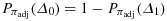
The probability that H₁ holds conditional on the impossibility of full extrapolation is denoted by 1 − q. Now the probability of H₁ can be written as

(4)

(5)

Note that s refers to the disbelief in the ‘similarity’ (scepticism) between the source and the target population, whereas 1 − q refers to the prior probability of no effect in the target population, if similarity cannot be applied as an argument: how likely is the alternative, if it is found that extrapolation regarding efficacy cannot be applied? One may tend to choose q values close to 1 in such a situation, but certainty with regard to existing differences between the population may not exclude that the drug is working in the subpopulation; hence, values of q < 1 may be reasonable. In particular, there may be some information from past use of the drug in the target population (e.g. from off-label use in the paediatric population). Under our proposed extrapolation assumption 3, a lower boundary seems reasonable for logical consistency. Otherwise, the belief in H₁ would be higher, if full extrapolation would be regarded as not applicable.

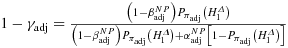
With the aforementioned assumptions and fixed q and s, this describes the α-level adjustment scenario, where a paediatric trial is designed to be conducted after a positive result in the corresponding adult trial. With particular values of q and s, a prior probability of the alternative hypothesis is given by equation 5, which will be denoted from now on. The corresponding positive predictive value, derived by the Bayes theorem will be written in a similar fashion as .

2.2 Evidence based α-level adjustment

We aim to derive a new test φ_adj with error rates α_adj and β_adj. This test should provide the same degree of belief , as a positive test result would provide in the benchmark scenario (=1 − γ):

(6)

If this equation holds, in our framework, we consider positive test results for φ_b and φ_adj to be equally convincing for regulators. By equation 6,

(7)

where, the left side of equation 7 refers to the benchmark scenario and α_adj and β_adj are chosen such that the equation holds. Clearly, the type II error rate should not be different from what is usually chosen from the sponsors (and regulators) perspective, because the main objective of the study is to obtain a positive result conditional on the true H₁, that is, β_adj=β. This means, that α_adj is the only remaining variable in 7, from which

(8)

for r ≠ 1 and is now easy to derive. Thus, the α level is raised by a factor, representing the ratio of prior odds in favour of the H₁ in the α-level adjustment scenario and in the benchmark.

By using 5, equation 8 can be written as

(9)

In the last equation, is the α-level adjustment factor, which after fixing γ only depends on r, q and s. By using 1 − γ from the benchmark scenario, we see from equation 9 that for s→0, the α-level adjustment factor approaches , so that the maximum value for α_adj is 1 − β. Note that a test with a level of 1 − β has a constant rejection probability of 1 − β irrespective of the null hypothesis or the alternative being true. Such a test refers to full extrapolation, because in theory a test with this property can be achieved with a sample size of zero by simply running a Bernoulli experiment with p = 1−β. No evidence is necessary also for the case q = γ, as α_adj again takes its maximum value 1 − β. For s→1, α_adj approaches and hence approaches α for q = r: in case of full scepticism about the similarity (s = 1), the only prior information on H₁ to be used is the belief 1 − q. If 1 − q = 1−r, we simply end up with the test in the benchmark scenario (φ_adj=φ_b). An interpretation for this particular case q = r is that early phase data in the paediatric population are available such that we are in the same situation as if we were starting a regular phase III drug development programme in the source population.

In Table 1, the values of the α-level adjustment factor are calculated according to equation 9 for different values of s, r and q. With decreasing s, increases. For fixed s and r, this factor also increases with decreasing q. When only r is allowed to vary, then an increase of r leads to an increase of . Note that the maximum inflation factor of 909.86 (r = 0.75, q = 0.1, s = 0.01 and γ = 0.0023) in Table 1 results in an increase of α = 0.025² to an α_adj of 0.57, which in practice would mean no further study in the target population.

Table 1. Different values of scepticism s (left column) motivate different values of for calculating .

0.9	10.10	4.55	2.70	1.78	1.22	0.85	0.59	0.39	0.23	0.11
0.8	11.48	5.24	3.16	2.12	1.50	1.08	0.79	0.56	0.39	0.25
0.7	13.24	6.13	3.76	2.57	1.86	1.38	1.04	0.78	0.59	0.43
0.6	15.58	7.31	4.55	3.16	2.33	1.78	1.38	1.08	0.85	0.67
0.5	18.85	8.96	5.65	3.99	2.99	2.33	1.85	1.50	1.22	1.00
0.4	23.71	11.43	7.30	5.23	3.99	3.16	2.57	2.12	1.77	1.50
0.3	31.74	15.52	10.04	7.30	5.64	4.54	3.75	3.16	2.70	2.33
0.2	47.50	23.62	15.50	11.40	8.94	7.29	6.11	5.23	4.54	3.98
0.1	92.51	47.32	31.58	23.57	18.73	15.48	13.15	11.39	10.03	8.93
0.08	113.82	58.85	39.47	29.57	23.56	19.53	16.63	14.45	12.75	11.39
0.04	209.96	113.41	77.49	58.74	47.22	39.42	33.79	29.54	26.22	23.55
0.02	361.90	209.28	147.03	113.21	91.97	77.40	66.77	58.68	52.32	47.18
0.01	566.12	360.89	264.72	208.94	172.51	146.86	127.81	113.11	101.42	91.91
	(a)r = 0.5, 1 − γ = 0.9992
0.9	3.37	1.52	0.90	0.59	0.41	0.28	0.20	0.13	0.08	0.04
0.8	3.83	1.75	1.06	0.71	0.50	0.36	0.26	0.19	0.13	0.08
0.7	4.42	2.05	1.25	0.86	0.62	0.46	0.35	0.26	0.20	0.14
0.6	5.21	2.44	1.52	1.05	0.78	0.59	0.46	0.36	0.28	0.22
0.5	6.32	3.00	1.89	1.33	1.00	0.78	0.62	0.50	0.41	0.33
0.4	7.97	3.83	2.44	1.75	1.33	1.05	0.86	0.71	0.59	0.50
0.3	10.71	5.21	3.36	2.44	1.89	1.52	1.25	1.05	0.90	0.78
0.2	16.16	7.96	5.20	3.82	2.99	2.44	2.04	1.75	1.52	1.33
0.1	32.25	16.14	10.69	7.95	6.30	5.20	4.41	3.82	3.36	2.99
0.08	40.14	20.20	13.42	10.01	7.95	6.58	5.59	4.86	4.28	3.82
0.04	78.16	40.09	26.88	20.18	16.13	13.41	11.47	10.00	8.86	7.95
0.02	147.68	78.06	52.98	40.06	32.18	26.87	23.06	20.18	17.93	16.13
0.01	265.36	147.51	102.09	78.01	63.10	52.96	45.61	40.05	35.68	32.17
	(b)r = 0.25,1 − γ = 0.9997
0.9	30.25	13.65	8.10	5.33	3.66	2.55	1.76	1.17	0.70	0.33
0.8	34.28	15.70	9.48	6.36	4.49	3.24	2.35	1.68	1.16	0.75
0.7	39.44	18.32	11.24	7.69	5.55	4.13	3.11	2.35	1.76	1.28
0.6	46.24	21.81	13.58	9.45	6.97	5.31	4.13	3.24	2.55	1.99
0.5	55.65	26.66	16.85	11.91	8.94	6.96	5.54	4.48	3.65	2.99
0.4	69.49	33.86	21.71	15.59	11.90	9.43	7.66	6.33	5.30	4.47
0.3	91.89	45.69	29.75	21.67	16.79	13.52	11.18	9.42	8.04	6.95
0.2	134.32	68.69	45.51	33.65	26.46	21.62	18.15	15.54	13.50	11.86
0.1	245.37	132.88	90.52	68.30	54.61	45.33	38.62	33.55	29.58	26.39
0.08	293.30	162.52	111.83	84.91	68.22	56.85	48.61	42.37	37.47	33.53
0.04	479.54	290.63	208.01	161.68	132.03	111.43	96.28	84.68	75.50	68.06
0.02	700.68	475.98	360.05	289.30	241.63	207.33	181.46	161.26	145.05	131.75
0.01	909.86	696.89	564.50	474.22	408.73	359.04	320.05	288.65	262.81	241.17
	(c)r = 0.75, 1 − γ = 0.9977

• The error rates α and β from the benchmark scenario are considered to be 0.025² and 1 − 0.9²=0.19, respectively.

3 Extrapolation in normally distributed data

In this section, we propose a generalized framework for the test of one-sided hypotheses by introducing general prior distributions. Then, we motivate the application of two-point priors and focus on the special case of normally distributed outcome variables.

Let π denote a prior distribution on a parameter Δ and φ denote a test procedure testing H₀:Δ≤Δ₀ against H₁:Δ > Δ₀.

where and P(φ = 1|Δ) denotes the probability of a rejection given Δ. The left-hand side in the first inequality is the Bayesian power, defined as the average of the frequentist power across alternatives according to the prior π. In the same sense, a Bayesian type I error rate can be defined as .

Similar to our model in the last section, we now take a look on the two scenarios, the benchmark and the α-level adjustment scenario.

Benchmark scenario:

Let π_b represent the prior belief in this scenario and with error rates and denote a standard trial in phase III that is usually chosen to be equivalent to a Neyman–Pearson test. The posterior belief after rejection is then given by

where is the subset of H₁ that is considered to be non-relevant for the Bayesian power calculation.

The question is now how to choose π_b because different opinions about the effect Δ lead to different posterior knowledge of the H₁. Our suggestion is as follows: similarly to the formulation of the benchmark scenario in the previous section, we first fix the prior probability 1 − r, but this time this value represents the belief on the parameter set . In the Appendix, we will show, that every prior π_b fulfilling leads to a positive predictive value with the property

The right-hand side of this inequality can be thought as the positive predictive value of the test coming from a Dirac distribution π^NP(A) = r·1_{A}(Δ₀) + (1 − r)·1_{A}(Δ₁)(here, 1 denotes the indicator function). It furthermore holds

With the last two inequalities, we can conclude that after the choices of and 1 − r, both the Bayesian power and the positive predictive value are controlled on a level and on a level 1 − γ_b respectively with , for the set of all prior distributions π_b with .

Note that in the benchmark scenario, the restriction on two points in the parameter space is widely used when planning a frequentist phase III study at a level α and a power of 1 − β, so that focusing on these two points is not an uncommon approach.

α-Level adjustment scenario:

Similarly to the restriction of possible prior distributions in the benchmark scenario to such priors π_b that fulfil the constraint , we will restrict the possible prior distributions π_adj in the α-level adjustment scenario. To this end, we repeat the approach from the last section as follows: if full extrapolation can be considered as possible, all the evidence can be taken from the source population; hence, . Furthermore, has to be specified. After specifying the scepticism s, this again leads to

as in equation 5, which we will use as a condition for the priors π_adj in the α-level adjustment scenario.

By again defining a Neyman-Pearson test with error rates and and , as in the benchmark scenario, it can be concluded that the Bayesian power is controlled at a level and the positive predictive value

is controlled at a level 1 − γ_adj with . Therefore, we again calculate the positive predictive value of the Neyman–Pearson test with prior probabilities coming from a two-point distribution with probabilities and to derive a lower bound for the positive predictive value under constraint (Appendix).

Given our prior assumptions in both scenarios, we aim to control the positive predictive value and the Bayesian power in the α-level adjustment scenario at the level 1 − γ_b defined in the benchmark scenario. To that end, we equate the lower bounds of the positive predictive values in both scenarios 1 − γ_b=1 − γ_adj, which can be written as

This is exactly of the form of equation 7, and hence, for equal type II error rates , all the results from Section 2 can be applied directly.

As an example, we now show how the previously developed framework can be applied in the setting of normally distributed outcome variables (variance known). We consider two groups of patients, where the first group receives an experimental treatment (T) and the second group acquire either the standard clinical intervention or a placebo (C). 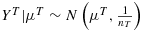For n_T measurements in the experimental group, and n_C measurements in the control group, and denote independent estimators for the respective group mean. In this setting, the variances for the observations are assumed to be known and equal in both groups, and the measurements are given in units of this variance. Our interest lies on the effect of the experimental treatment Δ = μ^T−μ^C, which can be estimated in a natural way by , where . For our test problem, we consider the null hypothesis H₀:Δ≤Δ₀ and its alternative H₁:Δ > Δ₀. With the following rejection rule, φ = 1 if and only if

(10)

for specific α, n and where x_n denotes a realization of X_n, we have the classical test that controls the type I error rate at level α. The power is controlled by an adequate selection of n.

In Figure 1, the fractions of the adjusted sample size based on α_adj over the standard sample size are drawn for different values of s, q and r = 0.5. Here, the formulae with A = α_adj for n_adj and A = α = 0.025,0.025² for n were used, with a targeted power of 1 − β = 0.9 and 1 − β = 0.81, respectively.

At first, we realize that for decreasing q (more prior belief in the alternative if extrapolation is not assumed to be a possible option), the decrease in sample size becomes larger. Moreover, for q = 0.5, even large scepticisms (s > 0.5) may lead to a saving of sample size. Savings of sample size (values below the horizontal line) are possible up to scepticism values similar for high or low significance levels. Note that if the scepticism is high, that is, putting more prior belief in the non-applicability of extrapolation and/or in the lack of efficacy if extrapolation is not considered to be an option in our framework, larger sample size than in the conventional test may be required to achieve the same high positive predictive value in the end. The possible savings however are larger for the higher significance level 0.025 (left panel in Figure 1). For the lower significance level (right panel), the sample size decrease is very steep for very small scepticisms.

3.1 Rejection probabilities

In Figure 2, curves for the rejection probabilities in the aforementioned discussed two-sample normal distribution scenario with common σ = 1 are drawn as a function of the true effect Δ. The α level in the benchmark scenario is set equal to 0.025 in Figure 2(a) and 0.000625 in Figure 2(b). In these two figures, the relative sample sizes were calculated to reach a power of 0.9 and 0.81, respectively, at the alternative Δ = 1. The reference for calculating the relative sample size is a traditional parallel group comparison with α = 0.025 with 1 − β = 0.9 (Figure 2(a)) and α = 0.025² with 1 − β = 0.81 (Figure 2(b)), respectively. Curves are drawn for a scepticism s equal to 0.1 (dark grey), 0.3, 0.5, 0.7 and 0.9 (light grey). In both figures, 1 − r takes values of 0.75 (top line of plots), 0.5 (second line) and 0.25 (bottom line of plots). In the first, second and third columns, 1 − q is set to 0, 0.25 and 0.5, respectively.

A decrease of q as well as an increase of r increases the α-level adjustment factor and therefore decreases the needed sample size in our approach: the relative sample size as compared with the reference design is <1. This is in complete accordance with the results already discussed for the framework of simple null and alternative hypotheses in Section 2.

Figure 2 also illustrates the risk of erroneously relying on extrapolation. Let us assume that for the paediatric population, there is no effect at all (H₀ is true). Obviously, the probability for a false positive claim in the paediatric population when applying the adjusted test is α_adj. This can be considerably large for large 1 − q, the prior belief in efficacy of the paediatric drug if extrapolation is not deemed to be feasible, or small scepticism s (high confidence in similarity). Somehow counter-intuitive is the impact of 1 − r: the smaller the belief in the alternative in the benchmark scenario, the larger the false positive rate α_adj in the adjusted test. This is because with increasing values of 1 − r, the level of evidence 1 − γ reached in the benchmark scenario is also increasing (see the left side of equation 6). If on the other hand the alternative is in fact true, then the power is 1 − β by design (Figure 2).

4 Example: the Food and Drug Administration decision tree

In a recent review 15, it was shown that 68% of 166 paediatric products investigated used the concept of partial extrapolation. This indicates a high confidence of experts that adult data can be extrapolated to some extent to the paediatric population. Full extrapolation was only applied for 14% of the products, which corresponds to a scepticism equal to 0 in our framework. The supplementary material of the review contains tables listing the indications, the age groups and the products, for which no extrapolation, partial extrapolation or full extrapolation have been applied. However, there is no quantitative description on the amount of scepticisms leading to different study programme reductions. We tried to give a rough visualization of the decision tree in terms of our framework based on scepticism. In Figure 3, the horizontal lines indicate the three levels of evidence, and the lowest bar refers to two independent trials, both on a one-sided significance level of 0.025. To apply our previous framework, we assumed instead that a single trial with a significance level of 0.025² would be performed. The middle bar corresponds to a single trial at a one-sided significance level of 0.025; the highest point indicates full extrapolation (no clinical trial needed). To mimic the FDA decision tree, the length of the bars for the distinct significance levels have been chosen in a somehow demonstrative way such that the curve for the adjusted significance level crosses the central bar right in the middle. We believe, that this is a fair approximation of the curve sharing a fixed initial point and two piecewise constant levels. It should be noted, that our proposal could be interpreted as a continuous generalization of the three levels of the FDA decision tree, assuming that they correspond to three discrete levels of scepticism.

Figure 3 shows a sharp increase of α_adj with decreasing scepticism s in the relevant regions where the decision has to be made whether one or two pivotal studies have to be performed. Small differences in the assessment of s may have substantial consequences for the paediatric development programme. The figure also shows that to achieve the same posterior probability for a relevant effect size, full extrapolation (highest point at the left) is possible only if the experts are completely certain that extrapolation is fully applicable (s = 0). But also relaxing the drug development to a single trial at level 0.025 (middle bar) according to our framework and graphical approximation would require a very high belief in extrapolation (in terms of a small s). This seems to be the case for most of the products in the experience of the FDA 15. If there is some belief in efficacy if extrapolation is not considered to be possible (q < 1), slightly larger scepticisms may allow to avoid the full development programme (for the FDA following the two pivotal studies paradigm).

5 Discussion

In drug development, several standards have evolved over time. Most of the statistical standards refer to the planning and analysis of single trials (e.g. 16). The important quality of reproducibility of trial results for long time has been accounted for particularly at the FDA demanding the two pivotal studies paradigm for phase III of drug development 17. However, it is also possible to rely on a single adequate and well-controlled study of a drug, if supported by additional evidence from other sources 17-19. For drug development in small populations 8, to keep such standards may simply not be feasible. For subpopulations, such as the paediatric population, an additional problem arises because when developing a drug for children, in general, sufficient data are available from clinical trials having been performed for authorization of the drug in the adult population. In this situation, parents will be very cautious to allow their children to participate in paediatric trials, particularly in trials using a placebo control that will be excluded in life-threatening diseases anyway. There is a never ending discussion if placebo-controlled trials may be performed at all in paediatric populations when the drug has been registered for adults. The consequence of all the ethical, feasibility and economic constraints in the past was that only a small proportion of drugs registered for adults have been also registered in children. Off-label use of the drug in children was the consequence if paediatric doctors believed that the drug would improve their patients' health. Shifting such decisions to the responsibility of the individual paediatrician without any access to systematic collection of efficacy data in the paediatric population is not an acceptable option from the legal and medical perspective. Hence, the legislation has been changed. According to this new legislation, a new drug for adults is only registered at the FDA or EMA when a programme for drug development (at the EMA a PIP) in children has been provided by the drug developer and has been approved by the regulators (at the EMA by the Paediatric Committee). To not to be late with the registration in children, the development programme has to be proposed already early in the development programme for adults. Another advantage of an early development plan for children is that at this time it could be integrated scientifically in the adult development by planning studies in adults that in turn provide specific data relevant for the paediatric development. This is the crucial problem: the earlier a paediatric programme is planned, the less information is available from adults. Hence, expert knowledge on the type of disease and type of drug plays an important role in early deciding on the design of a paediatric development programme to be accepted by regulators. Similar arguments may apply for very rare diseases where full programmes are infeasible or could withhold the beneficial use of a potent drug for a long time. Moreover, at the end of an overly long development programme, there could be no more interest in the drug because other potent therapeutic options have been established meanwhile.

We have tried to structure this procedure to decide on a drug development programme under uncertainty. Two quality criteria to compare different drug development programme have been fixed: first, the power of detecting an effective drug in the end is prefixed at a certain value. This is in the interest of the developer. Second, the posterior probability that there is indeed a relevant positive treatment effect, after the test of the no effect null hypothesis has been rejected, is also fixed at a (large) value. This in our framework is in the public interest of the regulator who aims at a large positive predictive value of the final test decision. As a paradigm for standard drug development, we used a conventional clinical trial in phase III analysed by a statistical test with significance levels 0.025 or 0.025² and a certain prior belief (1 − r) in effectiveness based on earlier phases before starting phase III. In contrast, we looked at a test with an adapted significance level, where the adjustment of the significance level is depending on the prior belief on the possibility of full extrapolation from another source (e.g. from another population). Not surprisingly, noticeable sample size savings are only possible if the prior belief in efficacy is fairly high. We looked also on how the results would change when we assume that there is still a positive belief (1 − q) in efficacy although extrapolation is not considered to be applicable. Obviously, the opening of a new track for a positive result by choosing q < 1 will increase the savings in sample size.

With regard to the FDA decision tree for extrapolation to paediatric populations (full extrapolation, a single trial and two pivotal studies) to apply full extrapolation, we need complete confidence in extrapolation. The reason is that a standard programme of drug development with a reasonably high power (e.g. 0.9) and plausible prior odds of 1 (r = 0.5) results in very large positive predictive values given the programme has succeeded to reject the null hypothesis of no efficacy (0.973 for a test at level 0.025 and 0.999 at level 0.025²). If no trial is run, there should be no doubt at all in the appropriateness of extrapolation in order to end up formally with a positive predictive value of the magnitude in the benchmark scenario. But even for relaxing the statistical rigour to the degree that only a single trial at a conventional significance level has to be run, the scepticism about the appropriateness of extrapolation has to be very small. It will be difficult to settle on such borderline prior beliefs in expert panels accounting for potential differences in eminence-based information. Moreover, as also pointed out in the reviewing process, the approach ‘is highly dependent on a number of assumptions related to the key parameters used to determine the adjusted level of α for the target population’. In Figure S1 of the Supporting Information, we present results of a sensitivity analysis, quantifying the impact of varying assumptions on the relationship between α_adj and s within our simple framework. Here, we also look at the situation, where the assumption of equal levels of evidence and equal power in the adult and paediatric programme is dropped. The relationship varies considerably with varying probability 1 − q of effectiveness without the option of extrapolation, and with varying levels of evidence 1 − γ_c to be reached in the paediatric study programme (dropping the assumption of equal level of evidence for adults and children in equation 3). To understand the high dependency on 1 − γ_c, it is helpful to look at the level of evidence in terms of odds: assuming 1 − γ_c=0.9 the corresponding odds in favour of the alternative against the null hypothesis are 9:1, whereas for 1 − γ_c=0.9992 in the two-pivotal study programme, the odds are 1249:1. Less variability is observed when the power in the paediatric study programme 1 − β_c is chosen differently to that in the adult population. Variation of the targeted level of evidence in the adult population 1 − γ_a does also not severely impact on the relationship.

A common regulatory practice to ask for a single study in the paediatric population would – in our framework – correspond to low scepticism of experts about the appropriateness of extrapolation from the adult population. To this end, it seems to be questionable, in particular with regard to the significance level 0.025²(which mimics the two pivotal studies paradigm of drug regulation), whether the α-level adjustment approach in small populations is a feasible way from the perspective of the responsible experts who have to decide at an early stage of the drug development process. In very small populations, this will have to be further relaxed for feasibility reasons, so that only smaller positive predictive values following a successful development programme will be achievable. Such a relaxation, in combination with post-marketing research, may be very reasonable in indications were no accepted efficacious therapy is available. One of the purposes of this paper is to bridge frequentist and Bayesian arguments and create a framework to compare different approaches and counter weight evidence from data in (smaller) trials and eminence (expert knowledge) in this specific environment of decisions under uncertainty in medicine. The importance of decisions on extrapolation, for example, in the paediatric population can be seen from the review 15.

A methodological spin off in our framework is that simple two point priors may be used in the argumentation as they, under some constraint, have some useful limiting properties among all other prior distributions. It should be noted that we tried to use our framework to portray existing decision structures in drug regulation. However, it could also be used in different contexts, for example, fixing the positive and negative predictive values of regulatory decisions, including utilities/losses or simply backward calculating a ‘virtual’ scepticism if only a small sample size in the target population is available and cannot be based on calculations with a targeted power. It has to be stressed that our framework refers to a very early phase of drug development in the target population: on the one hand, it is understandable that regulators aim at binding commitments of drug developers on which and how much evidence will be supplied for the registration of a new drug in children. In the present legislation, such a commitment is even a condition for registration of the drug in adults. On the other hand, the actual trials in the paediatric population are often starting not before or even quite delayed after the drug has been registered in adults. Hence, the environment of extrapolation is likely to change if data from adult studies will become available. Consequently, by the logic of science, it is reasonable to consider adaptations of the agreed paediatric development programme. In the legislation, the request for modification of an approved PIP, in the EU to be dealt with by the Paediatric Committee of the EMA, is an appropriate way to deal with this learning from experience situation. Other Bayesian approaches using data from the source population 20-23 may be applied to adaptively modify the preplanned paediatric development programme. This may be achieved in practice by allowing for the option of an adaptive PIP as an example of an adaptive licensing approach 24. It seems to be reasonable that more emphasis in research and application should be put also on this stage of developing new drugs in children.