
The coronavirus disease (COVID-19) pandemic: simulation-based assessment of outbreak responses and postpeak strategies
Abstract
It is critical to understand the impact of distinct interventions on the ongoing coronavirus disease pandemic. I develop a behavioral dynamic epidemic model for multifaceted policy analysis comprising endogenous virus transmission (from severe or mild/asymptomatic cases), social contacts, and case testing and reporting. Calibration of the system dynamics model to the ongoing outbreak (31 December 2019–15 May 2020) using multiple time series data (reported cases and deaths, performed tests, and social interaction proxies) from six countries (South Korea, Germany, Italy, France, Sweden, and the United States) informs an explanatory analysis of outbreak responses and postpeak strategies. Specifically, I demonstrate, first, how timing and efforts of testing-capacity expansion and social-contact reduction interplay to affect outbreak dynamics and can explain a large share of cross-country variation in outbreak pathways. Second, absent at-scale availability of pharmaceutical solutions, postpeak social contacts must remain well below prepandemic values. Third, proactive (targeted) interventions, when complementing general deconfinement readiness, can considerably increase admissible postpeak social contacts.
© 2020 System Dynamics Society
Introduction
On March 11, the World Health Organization declared the coronavirus disease (COVID-19) outbreak a global pandemic (WHO, 2020a). As of mid-May, over four million cases of COVID-19 virus infections and over 300 thousand deaths have been reported (Roser et al., 2020). While the disease has affected over 200 countries, areas, and territories, outbreak patterns and responses have varied widely (Cohen and Kupferschidt, 2020). In Singapore, extensive restrictions on movement started 3 days after the first discovered case (Xianbai, 2020), whereas other countries have been slower to reduce social and economic interactions. South Korea deployed rapid and large-scale testing across the population, while the United States has initially been slow to build up testing capacity (Cho, 2020). Across Europe, responses have also differed considerably (Politico, 2020). On March 16, the French government ordered citizens to stay at home except for essential activities (Erlanger, 2020). In contrast, the U.K. government initially suggested avoidance of public places (Triggle, 2020), yet bars, restaurants, and museums remained open. Prime Minister Boris Johnson subsequently changed course, but confusion persisted over what was and wasn't allowed (Mason, 2020). The same virus and disease, different government and citizen responses.
Early data on the pandemic (Roser et al., 2020) suggested the vital importance of rapid scaling up of testing and interventions aimed at reducing physically proximate interactions (“social contacts”) for decreasing total and peak infections. But the different approaches and pathways across countries raise a number of critical questions, including: How do these various interventions impact the outbreak patterns? Why is large-scale and early testing so important? What is the differential effect between enforcing or discouraging social-contact reduction? How sensitive are interventions to imperfect compliance by citizens? How do different interventions interact to alter outbreak patterns? How much can restrictions relax once the outbreak is under control? How important are targeted interventions? And, what is the importance of coordinating and aligning efforts across countries? Answering such questions requires detailed understanding of the underlying drivers of the dynamically complex diffusion patterns of infectious diseases involving not only virus transmission but also the ways in which, in response to an outbreak, populations may alter their social contacts, health experts expand testing and reporting, and policymakers implement social-distancing and surveillance policies.
The central purpose of the behavioral dynamic infectious-disease policy model I develop here is to analyze the individual and joint impact of diverse, specific public health control measures over the epidemic cycle, including first outbreak response, first-wave deconfinement, and virus resurgence. To capture critical virus and transmission characteristics (e.g. transmission rates and incubation and infectious periods), the model follows the principles of the widely used class of epidemiological Susceptible-Infected-Recovered (SIR) compartment models (Brauer and Castillo-Chavez, 2012). To represent the role of human responses to the outbreak and how these in turn alter the outbreak dynamics (Ferguson et al., 2020), the model also follows principles of behavioral dynamic modeling (Sterman, 2000). Within the field of system dynamics, a long history of compartment-based infectious disease models exists that takes such an approach (Darabi and Hosseinichimeh, 2020; Thompson and Duintjer Tebbens, 2008), studying issues ranging from pharmaceutical effectiveness in HIV/AIDS (Dangerfield et al., 2001), psychological factors in social-contact adjustment in Ebola (Pruyt et al., 2015), and to end-game strategies in the context of the poliovirus (Duintjer Tebbens et al., 2005; Thompson and Duintjer Tebbens, 2007).
Yet, while building on the fundamentals of these two research streams, policy relevance requires attention to issues central to the ongoing COVID-19 outbreak. For example, the current outbreak is characterized by high first-wave virus-transmission rates, by relatively high death rates for the severe, high-symptom cases accompanied with abundance of mild, low-symptom cases that allow largely undetected spreading (Ferguson et al., 2020; Kissler et al., 2020a). Further, presently there is much uncertainty about timelines of vaccination development and deployment as well as about immunity duration (Kissler et al., 2020a). Therefore, managing the COVID-19 outbreak requires not just end-game strategies but also effective nonpharmaceutical strategies including for deconfinement and outbreak resurgence.
To capture first-wave and postpeak dynamics for COVID-19, the core of the model forms a “susceptible exposed infectious recovered” (SEIR) model (Hethcote, 2000). The model further includes endogenous social-distancing responses by citizens and interventions by policymakers as well as the build-up and execution of case testing and reporting. Importantly, within the model, as in real life, citizens and policymakers respond to reported data of tested—not actual—positive cases during a progressing virus outbreak. Testing capacity, initially nonexistent, has to be built up. Further, the model differentiates mild cases—exhibiting mild symptoms or being fully asymptomatic—from severe cases. Because the former group is generally less likely to be tested but nevertheless infectious, this differentiation affects case detection and citizen responses and therefore the overall outbreak pathways. The model explicitly captures both symptom-based (reactive) testing and field-based (proactive) testing approaches as well as different types of interventions, including social distancing of the general population, home confinement of suspected cases, and quarantining of positive (detected) cases. The model structure has some generality in the sense that one can alter assumptions about virus-transmission parameters, citizen and policy behavior, and sociodemographic and geographical characteristics within and across segments.1 The model tracks key epidemic variables over time (e.g. the population within the various epidemic stages, the reproductive number—the average number of secondary cases that one case generates over the course of its infectious period), as well as clinical (e.g. hospitalizations, deaths) and behavioral variables (e.g. degree of social contacts and home-confined population reported versus actual cases).
I use the model to examine effectiveness of interventions to manage different phases of the COVID-19 pandemic. To do this, in the first experiment, I develop a baseline simulation run that calibrates the model against the rapidly developing data and literature on the ongoing outbreak (Dong et al., 2020; The Lancet, 2020; Roser et al., 2020). The parameters for the baseline are estimated through a cross-sectional calibration to time-series data (31 December 2019–15 May 2020) on reported cases and deaths, tests performed, and social-contact proxies for six different countries varying in their outbreak paths and intervention choices (South Korea, Germany, Italy, France, Sweden, and the United States). I then use the calibrated model to perform explanatory analyses within four additional experiments. First, I examine sensitivity of outcomes to individual- and multiple-policy responses. Next, I examine, within a more stylized context, the consequences of efforts and timing to deconfine and interventions that help reduce virus resurgence. In the final experiment, motivated by the large variation in clinical outcomes across countries, I examine in more depth the impact of heterogeneity in sociodemographic-related (e.g. age) vulnerability to the virus on the overall outbreak dynamics.
The analysis results show, first, how timing and extensiveness of testing and of social-contact reduction measures interplay and can explain a great share of the differences in outbreak pathways across countries. More quantitatively, while noting limitations in the degree of confidence in some of the specific parameter values and trajectories at this point during the outbreak, sensitivity analysis in the case of the United States suggests that a one-week earlier (later) ramping up of either testing capacity build-up or of social-distancing action could have led to the order of 50 percent fewer (additional) actual deaths. These large effects result in part from strong interactive effects involving multiple coupled positive feedback loops. For example, testing efforts do not only allow case identification and isolation but also help, due to increased awareness of the outbreak, accelerate interventions aimed at general contact reductions. Second, I show how countries, once falling behind in curtailing the outbreak, have difficulties catching up. Once the gap between tested and actual cases expands, a positive feedback involving transmissions from unidentified cases drives efforts toward reactive and late-stage, rather than proactive and early-stage, case detection. Third, in terms of deconfinement strategies, I show that, absent at scale availability of pharmaceutical solutions, risks of renewed large-scale outbreaks are very high when social-contact rates exceed 60–70 percent of the prepandemic levels. Those risks depend importantly on a country's preparedness for deconfinement that includes confinement policies prior to deconfinement. Specifically, the presence of effective and extensive targeted testing and intervention approaches—suspect case identification through contact tracing and testing, as well as suspect case isolation, surveillance, and isolated case compliance—are vital to reduce the multifaceted risks and impacts of resurgence. Fourth, as a more general finding, the model allows pinpointing the origins of the fundamentally complex dynamics of infectious diseases caused by both virus transmission and human behavior. Powerful positive feedbacks that accelerate infections combine with delays in infection detectability, inertia in the build-up of testing capabilities, and with challenges in rapidly limiting human contacts. In capturing responses behaviorally and including important delays and interdependencies, the model further helps explain why and how swift and comprehensive responses can reduce the impact of epidemic outbreaks. In clarifying these endogenous dynamics, our model provides insights that are fundamentally different from and complement policy models that study interventions as exogenous shocks (Kissler et al., 2020b). By allowing the exploration of different intervention strategies with endogenous behavior—from social-distancing advice to home confinement of suspect cases, I provide a general quantitative framework for better understanding under what conditions what combinations of measures help suppress the epidemic outbreak—at an early stage of an outbreak or postpeak.
In the remainder, I begin by providing a short background of the COVID-19 pandemic, describing the virus characteristics and varying outbreaks paths and responses within selected countries, and motivating the policy questions. I then highlight the model structure and discuss the key equations (as the full model is available in the online supporting information). Next, I perform a number of calibrated and stylized simulation-based experiments. The article concludes by discussing policy implications and methodological contributions and by suggesting follow-up work.
Background
The virus
From 31 December 2019 to 3 January 2020, 44 patients with pneumonia of unknown etiology were reported in China. On 7 January 2020, a new type of coronavirus was isolated by the Chinese Ministry of Health (WHO, 2020b). Soon the Chinese Ministry of Health reported the cases' exposure history to the Huanan Seafood Wholesale Market in Wuhan. The second week of January 2020, other countries identified confirmed cases related to traveling overseas, including Japan, Thailand, and South Korea. Reported cases went from over 150 thousand by mid-March to over 1.25 million on April 6, with over 65 thousand reported deaths in a total of 180 countries (Korean CDCs, 2020; Roser et al., 2020).
The virus causing the respiratory illness COVID-19, “severe acute respiratory syndrome coronavirus 2” (SARS-CoV-2, earlier provisionally named “2019 novel coronavirus” (2019-nCoV)), is thought to spread from person to person through droplets and contacts when a person with the virus coughs or sneezes and by touching objects contaminated with the virus, then touching one's eyes, nose, or mouth. (Hereafter, we solely use the acronym COVID-19, indicating both the virus SARS-CoV-2 and the disease COVID-19.) Main symptoms include those associated with respiratory infections, ranging from mild to severe, such as fever, malaise, cough, shortness of breath, and pneumonia. In addition, phlegm, sore throat, headache, hemoptysis, nausea, and diarrhea also appear. Elderly, immunocompromised patients, and patients with underlying medical comorbidities are most likely to be in critical condition or die from the virus. Early estimates suggest a crude case fatality rate for COVID-19 of about 1–2 percent (Shim et al., 2020; WHO, 2020b), much larger than the order of 0.1 percent for a moderate seasonal influenza. Yet, there is still much uncertainty about the true infection fatality rate (IFR)—of actual cases. Deriving this requires information about the actual number infected (the denominator), but this is challenging because the often-limited testing capabilities and because endogenous factors such as hospital overload affect mortality risks (Ghaffarzadegan and Rahmandad, 2020). The IFR is particularly hard to detect because of the large number of cases with mild and/or flu-like symptoms. For example, some studies suggest that about 80 percent of people with COVID-19 have mild (or no) symptoms, while 20 percent have severe symptoms, with about a third of those latter groups becoming critically ill (ECDC, 2020).
The extent of an epidemic outbreak is affected by key virus-transmission parameters. Estimating values of parameters such as infectious contacts and duration of infectivity is of critical interest to those seeking to impact this (Anderson et al., 2020). Compared to Influenza or Ebola, transmission is rapid due to high infectivity. The duration of the infectious period for COVID-19 is estimated to be 5 to 10 days (Zou et al., 2020), after an incubation period of 2 to 14 (5.5 average) days (Li et al., 2020). The fundamental metric transmissibility of a virus, the basic reproduction number R0—representing the number of people infected during once infectivity at the first infection—is estimated to be on the order of 2.4–3.3, quite higher than that for seasonal flu or Ebola (Chowell et al., 2004) but lower than for severe acute respiratory syndrome (SARS) (Lipsitch et al., 2003; Read et al., 2020; Walker et al., 2020). Estimates using this reproduction number suggest that globally, an unmitigated COVID-19 epidemic would lead to about seven billion infections (Walker et al., 2020). Given the case fatality estimates, this could potentially result in 40 million deaths.
An unmitigated scenario, while important as reference, is unrealistic because transmission rates decline as governments and citizens respond as reported cases and deaths accumulate, leading to reduced contacts. Yet, both outbreak patterns and responses varied greatly across countries.
Varying outbreak pathways and responses
Responses in Asia (South Korea, Hong Kong, Singapore, Mainland China, and, to some extent, Japan) show that active policy measures such as quarantine, social distancing, and isolation of infected populations can contain the epidemic (WHO, 2020b). While the outbreak has been contained within multiple countries through early government action and through social-distancing measures taken by individuals, in many other countries, this has not been the case.2 To illustrate, consider the outbreak and responses in three countries across three continents: South Korea, Italy (the first known epicenter in Europe), and the United States (Figure 1). The four graphs show cumulative reported cases (per million people, pmp), cumulative tests performed (pmp), and two metrics of relative social contacts (mobility and school closings), starting from 31 December 2019 (the day of the first case reported to the WHO) until 15 May 2020.3 Across the three countries, the first reported cases occurred all within one day (19–20 January 2020, Figure 1, top left). Initially, reported cases were much higher in South Korea, suggesting it had become an epicenter. However, the fate of the countries differed considerably during the following 90 days: whereas in South Korea, reported cases stabilized around 200 pmp by early March; in Italy, by the end of March, it was at 1700 cases pmp; whereas in the United States, by the end of March, there were already 500 reported cases pmp. Case reporting, however, is not independent from case testing. In South Korea, it took 43 days to get from the first reported case to 2500 tests pmp (asterix), at which point there were 68 reported cases pmp. Italy reached 2500 tests pmp 15 days later, at 550 reported cases pmp. The United States reached 2500 tests pmp on March 27, 26 days later than South Korea, at which point there were 260 (steeply growing) cases ppm. With notable exceptions such as Iceland, testing has lagged in many other countries. In terms of social-contact reduction, South Korea, while not fully locking down, was also relatively quick to respond. This response is shown clearly in the mobility and school-closing graphs of Figure 1 (right). Italy, once containment efforts began, responded more extensively to reduce social contacts. Notably, the United States was slower and less extensive in its response. (Cyclical patterns have weekly frequencies reflecting natural workweek–weekend mobility variations. Note that the cycle amplitudes tend to attenuate during lockdowns.)

South Korea's approach reflects a more proactive approach beyond just testing. In particular, South Korea has focused on early detection of persons at risk and so to identify and then isolate the virus (Korean CDCs, 2020). As part of this, South Korea implemented a policy of early and widespread identification of suspected cases through targeted testing and isolation of “suspected cases”—family members and, through contact tracing, those who are thought to have been in close contact with positive cases. The quarantining and surveillance of positive and suspected cases involves following up those cases according to specific protocol and timing. Finally, efforts are done to build capacity of local government, build systems of cooperation between affiliated organizations, and educate and raise public awareness among the community (Korean CDCs, 2020). In Europe, confinement policies have been implemented but often much more slowly. Yet they have focused more on confinement of the general population. Italy's general lockdown commenced in the center and was gradually expanded to northern provinces (8 March). In the United States, despite urging from public health experts, by early April, some states and counties have taken limited action, with beaches and restaurants still open (Axelrod, 2020). Indeed, social activity has taken much more time to slow in Italy and the United States (Figure 1, top, showing mobility averaged across driving, public transport, and walking; and bottom, showing timing and extend of school closings).
Policy questions
These contrasting outbreak pathways and responses highlight the importance of aggressive and extensive testing and social distancing, often practiced in epidemic outbreaks (Jefferson et al., 2008). Further, because of the high basic reproduction number, relevant outcome measures are not only the total number of deaths but also, for example, the peak load of the health systems (Ferguson et al., 2020; Pueyo, 2020). During the first-wave COVID-19 outbreak, delays in testing and social distancing may greatly augment deaths, directly from increased COVID infections, and indirectly through the overburdening of the health system (Greenstone and Nigam, 2020). Adding to the complexity, while social distancing can come at a large societal and economic cost, limited social-distancing reduction or early deconfinement leads to resurgence risks (Eichenbaum et al., 2020). As countries have responded differently to the first wave and have begun making decisions toward deconfinement, it has become clear that their decisions are often influenced by complex pressures across realms—reports of reduced load on critical care units, economic actors with calls for opening business, frustrated citizens subjected to long-confined societal members, neighboring countries with their own actions. Finally, there are different ways to achieve goals. For example, what is the role of targeted approaches such as contact tracing, suspect case isolation, and community surveillance (Fraser et al., 2004; Wong et al., 2016). Altogether, the different decision-makers across the various countries face questions of what set of responses and their timings help manage the outbreak pathways, in the short and long run, and at what cost. Absent a thorough understanding of the dynamic interplays across virus transmission, citizen responses, and policy realms making an informed decision about altering—delaying, relaxing—interventions, individually or jointly, is impossible. A well-grounded dynamic integrative analysis is critical for developing such understanding.
Model
The computational model I outline here (Figure 2, high-level model overview) focuses on policy interventions for an infectious disease outbreak throughout the epidemic period, including deconfinement and resurgence. To capture virus-transmission dynamics, the core of the model forms an epidemiological compartmental SEIR structure commonly used by epidemiologists (Hethcote, 2000), with explicit times to symptom onset and infectiousness consistent with earlier epidemiological studies (Figure 2, top left panel). The model is also sensitive to the sociobehavioral complexity of policies and citizen responses with various ways to reduce social contacts of the general and infected population (Figure 2, bottom left panel). Policymakers decide about building case testing capacity and testing strategies including for targeted approaches that allow identification, testing, and surveillance of suspect cases within clusters (Figure 2, top right panel).

The model disaggregates the population across a number of dimensions related to virus transmission, disease symptoms, testing, and demographics (Figure 2, note on the bottom right). The demographic segments can be used to represent geographical regions (continents, countries, or provinces, etc.—as long as they are sufficiently large so that microlevel variation in individual contacts are less important) or sociodemographic heterogeneity (older versus younger populations; vulnerable versus less vulnerable groups) within a single geographic region. The model traces virus impact-related metrics such as reported and actual cases and deaths, as well as clinical and socioeconomic-related variables such as hospitalizations and social-contact reductions. Finally, a number of assumptions can be altered that affect the evolution of endogenous contacts and case testing and reporting within each segment, and through those, virus-transmission dynamics (Figure 2, bottom right panel).
In what follows, I highlight the key model concepts, structures, and variables. Likewise, the accompanying figures show simplified representations of the model sections. Appendix A.I in the online supporting information lists all model equations using the same sections and sequencing as below and provides additional visuals of the model structure.
Virus transmission
 and ced ′ d and on infectivity—the probability of infection given contact between a susceptible and an infectious person. Then, the virus transmission (in simplified form)4 is given by the following:
 (1)
(1)
Infectivity of the infected population, iid′, tends to be considerably higher than that of the exposed population, ied′. However, viral load measures suggest that in the case of COVID-19, infectivity commences before the onset of first symptoms (Ferguson et al., 2020; Pan et al., 2020; Zou et al., 2020;)—thus during the exposed period. Further, infectivity may vary across segments because regional climate (temperature/humidity) affects transmission (Xu et al., 2020; Kissler et al., 2020a).  and
and  equal within-segment contacts ced and cid, adjusted for relative cross-segment contacts
  For example, for the infected population:
 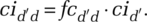 (We discuss the within-segment contacts below.)
After transmission, the population remains in the exposed state during a latent or incubation period λ, followed by the onset of the virus infection (Figure 3, Onset Rate from Exposed to Infected Population). At this point, symptoms (may) begin to show. Below outlines in more detail the disaggregated formulation of the infected state, including those parameters marked in Figure 3 with “*,” Finally, depending on the (true) infection fatality rate (IFR), those in the infected state either recover or die (Figure 3, right).
Infected population
The structure of the infected population is further disaggregated, most importantly to capture the role of large variation in symptoms across the populations. Only a small fraction of those infected exhibit severe symptoms (ECDC, 2020), and, because of that, detectability for a large part of the infected population is low (Figure 4). In the model, the fraction of cases severe fsd is defined as the fraction of all cases requiring some form of critical care. A share fhs of those with severe symptoms actually gets hospitalized, once they progress from early to advanced stage, after time to reach the advanced stage τa (Figure 4, top). Next, these severe-advanced cases either recover or die after a time to recover τrs, with the severe-case infection fatality rate ifrs being the actual (not reported) fatality fraction of the severe cases. Those with mild symptoms (Figure 4, bottom)—including a large share being fully asymptomatic—follows the same two-stage structure. However, none of those are hospitalized or die, so all recover after the recovery time for the mild population τrm. (Thus, the IFR equals ifrd = ifrs ∙ fsd.)

Social contacts
Virus transmission depends not only on exogenous virus-related transmission parameters but also on citizens and policymakers responding to an outbreak and taking measures to protect themselves or to curtail this outbreak. General population contact reduction may result from a range of responses and measures, including increased hand washing, mask wearing, physical distancing, prohibitions in gathering in groups, travel restrictions, school and nonessential office closings. Those exhibiting symptoms may reduce contacts by staying at home when feeling sick, irrespective of concerns about the virus outbreak, or may be ordered to self-isolate. Positive tested cases may be quarantined. As the population adjusts, social contacts, infectious contacts, and transmission rates change too.
In the model, social contacts of the infected population as well as of the general (and thus exposed) population reduce in response to the severity of a perceived outbreak in a number of different ways (Figure 5). The infected population may reduce contacts as: (a) positive tested population (detected cases)—at hospitals or elsewhere—are being quarantined (quarantining); (b) undetected cases exhibiting symptoms reduce their contacts voluntarily or urged by governments, beyond what they would otherwise do because of sickness (contact reduction); (c) undetected cases reduce contacts either voluntarily or being urged by governments (social distancing); and (d) undetected cases are being home confined because they have been associated with detected cases through targeted isolation efforts (home confinement). The exposed population may reduce contacts because: (i) undetected cases reduce contacts either voluntarily or by being urged by governments (social distancing); (ii) undetected cases are being home confined because they have been associated with detected cases through targeted-isolation efforts (home confinement).

 (2)
(2)where fci is the relative normal contact rate of infected population (compared to the normal contact rate of the general population).
Within-epidemic state contact reductions adjust to indicated levels over adjustment time τc. For example, social distancing for the infected population, isdd, adjusts to indicated general social distancing  ; thus
 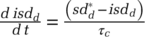 . Those quarantined and home confined adjust contacts as they are being transferred to their new epidemic state. Finally, those newly infected adjust their contacts to a level indicated by the infected population. This over-time contact adjustment of the newly infected population is captured through a coflow structure (Sterman, 2000).
 increases in perceived outbreak level od relative to reference outbreak level oref,d defined as the level at which any response commences, with sensitivity βsd,d and with maximum contact reduction sdmax,d:
 (3)
(3)This formulation implies that below the reference outbreak level oref,d there is no social-distancing effect. At oref,d the marginal responsiveness is maximal, subsequently decreasing asymptotically to sdmax,d. A greater βsd,d implies higher marginal individual responsiveness or larger populations.
As policymakers and citizens alter their behavior in response to the severity of the perceived outbreak and so affect virus-transmission rates, they respond to reported (not actual) data about positive tests and deaths. Media and experts report different metrics about the virus, but reported absolute cases and deaths tend to dominate the media and affect population behavior (Xiao et al., 2015). To be able to capture this, the model uses a general nonlinear classic CES formulation (McFadden, 1978). Formulating the respective impact of the reported cases and deaths as a non-linear weighted function may be relevant when the ratio of deaths and cases vary importantly over time or when comparing across different virus/diseases with varying infection fatality rates across them. However, for the analyses here, a simpler linear form satisfies, and the function is parameterized so to yield this special case. Therefore, effectively, the perceived outbreak level od is a simple weighted function of the reported deaths RDd and reported cumulative cases RCd, od = wd + (1 − wd)∙RCd with wd being the relative importance of reported deaths.5
Case testing and reporting
Case testing follows two main approaches: reactive and proactive. First, reactive testing is driven by the symptoms occurring under the currently undetected infected population Iiu (omitting demographic index d) within any of the states i either being mild m or severe s cases in the early e or advanced a, thus i ∈ {me, ma, se, sa} (Figure 4). Reactive testing occurs when the undetected population either self-reports their symptoms or is hospitalized with symptoms. The reactive testing process is identical across all states i (Appendix Figure A.1 in the online supporting information visualizes the testing process for the severe-advanced infected population Isa,u). Correctly identified positive tests tpi (hence, ignoring false positives) equal the fraction of actual cases tested ti times the case-detection fraction fd, and the fraction of actual tests being positive fpi (one minus the false negative fraction ffni, so fpi = 1 − ffni): tpi = fd · fpi · ti.The actual testing rate equals the desired testing rate constrained by effective testing capacity available for i, tcei. Hence, 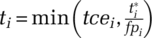 . Desired testing
  results from a fraction of the population Iiu reporting symptoms, of which a maximum fraction is deemed acceptable for testing, together captured by
  . Appendix A.I.3 in the online supporting information details the process including aggregation from and allocation of testing capacity across the different infectious states i). With the infectious cohort time τi,the indicated test rate for infectious population in state i is defined as
 , with Nfuthe relevant undetected exposed and infected population. The solution to this problem is:
 (4)
(4)where, as with reactive testing, proactive testing is constrained by the capacity, hence  . Nf is the effective pool within which to search. Because neither search type is close to random, Nf can be considerably smaller than the size of the population group within which the search is performed. We find Nf through the ratio of size of the undiscovered pool Nfu and the actual likelihood of finding a subjective case pf,
  .
.
 and for detection fraction fd,
 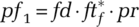 , with pr the random likelihood of encountering a single undetected infected person
  . The clustering parameter κf captures the effectiveness of proactive testing by indicating how efficiently “detectable cases” (those who have been infected by others) are actually identified and tested. A value of 1 implies effectiveness equal to random search. At small probabilities (pf′ ≪ 1), κf and pf interact linearly to increase the probability of success (pf ≈ κf · pf1) and thus proportionally decreases the effective search space
  . Generalizing the formulation, to ensure robustness for larger values of κf · pf, we get:
 (5)
(5)To illustrate the working of this expression, consider a population of N = 16M and Nu= 16k undetected cases in total (i.e. 0.1 percent of the population, so pf1 = 0.1 percent, assuming for simplicity fd · ftf = 1). Let Nfu=1000 of those cases exist within some known cluster of high infections, and tf=50 tests being performed within those known zones, with search time τt=1 day. Then, a targeted search effectiveness κf = 1 (random search) would give about 0.05 expected positive tests. Then, using the approximation  , κf = 12 implies that
  0.6 positive tests, while κf = 24 gives ≈ 1.2 positive tests, and κf = 480 gives about 23 out of 50 tests being positive. (When using the model Eqn 5 for pf, κf = 480 gives about 19 out of 50 tests positive—one can observe the diminishing returns in κf.) The value of targeted search effectiveness κf depends on conditions affected by social structures and mobility of the population as well as on the capabilities of experts in tracing actual positive cases within hot zones given such structures and mobility.
In addition, for contact tracing to be effective, a sufficiently large amount of positively tested cases needs to be traced. For sampling, simply Nsp,u = Iu + γe · E. For targeted testing, the pool of detectable infected population Ita,u depends on active work done to trace the tested population and identify potential suspect cases (Appendix A.I.3, Figure A.3, in the online supporting information). Thus, Ita,ubuilds with the detection of new cases tp, depending on the ability to identify associated cases through targeted testing fata as well as on the effective cases each infects, indicated by the reproduction number R. Thus, new detectable cases through targeted approaches build with 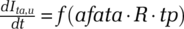 . The actual change rate is constrained by the undetected case pool size and involves an outflow proportional to the loss rate of undetected cases.
Testing capacity is constrained by availability and utilization of testing kits (See Appendix A.I.3, Figure A.4, in the online supporting information for the process). With initially a fixed number of kits TK0 (omitting index d) available, the building of testing kits TK begin when cumulative hospital visits associated with the virus symptoms exceed threshold level CH*, the building of additional kits begins, at growth rate g. The production of test kits continues until a desired level of testing capacity is achieved (cases/day/pmp). Utilization of test kits is a function of the growth rate of reported active cases: if reported active cases decline (increase), utilization reduces (increases). Finally, testing capacity is distributed across testing strategies, according to the following priority rule: (a) reactive—severe-advanced population; (b) reactive—self-reported symptom-based of early stage severe and mild cases; (c) proactive—field testing (targeted); (d) proactive—sampling.6
Quarantining and home confinement
Those who test positive are quarantined at quarantining fraction fqi, and thus move at rate fqi · tpi from undetected infectious Iiu to quarantined infectious state Iiq, while the remaining ones, (1 − fqi) · tpi, move to the detected (but not quarantined) state Iid. Home confinement of potential suspected (exposed and undiscovered infectious) populations builds from the stock of detectable cases for targeted testing. The stock of detectable cases accumulates in the same way as the pool of detectable infected population through targeted testing. The rate of accumulation is enabled by an ability to identify associated cases for home confinement, fahc. (For more details, see Appendix A.I.4, Figure A.5, in the online supporting information.) The actual home-confinement rate depends on the fraction of potential cases being home confined fhcd. This fraction builds as a function of perceived outbreak in the same way as social distancing (Eqn 3) and depends on the reference outbreak level oref,d, the maximum home-confinement fraction crhmax, and sensitivity parameter βcrh.
Analysis
The analysis section develops, through a number of logically ordered experiments, specific insights into first-wave outbreak and response dynamics and into postpeak confinement and resurgence strategies. In addition, the analysis serves to illustrate how the model can be used to enhance understanding of these problems more generally. The analytical strategy to present the results in the article involves, first, the construction and detailed analysis of a baseline case and, second, comparative analyses across alternative policy scenarios that each build on this baseline. The baseline is calibrated to the ongoing COVID-19 outbreak, using a cross-sectional dataset involving six countries, but also includes an out-of-sample counterfactual time segment. Experiment 1 examines, sequentially, the calibration results and the baseline case. Experiment 2 involves a sensitivity analysis of this baseline case, centered on policy and citizen responses to the outbreak within a subset of the countries. The next two experiments (3 and 4) involve an analysis about managing deconfinement and virus resurgence. We perform these using more stylized reference case that is derived from the baseline. The stylized context, while perhaps less relatable than a specific real-world case, allows for better comparability across results and in this way facilitates developing internally consistent explanations. This reference case stays as close as possible to the baseline. The final experiment, also using the stylized context, explores the relative effect of the virus on vulnerable populations by varying the symptom severity across population segments. For experiments 2 to 5, the variable “simulated actual deaths” (ADd) is the main outcome variable of interest.7
Experiment 1: baseline calibrated to the ongoing COVID-19 outbreak
To perform a cross-sectional calibration of the model, I constructed a country-level dataset with diverse outbreak data, including reported daily new cases, recovery rates, death rates, and testing rates, as well as a metric for social-contact rates. The dataset covers a large number of countries from 31 December 2019 through 15 May 2020.8 Daily reported new cases and deaths and testing data were retrieved from Ourworldindata.org (Roser et al., 2020). The metric for social contacts is proxied through a composite of data on mobility intensity—walking, driving, and public transport use—and on school closings (see Figure 1 for details and sources). Mobility and school-closings data have equal weight in the proxy for social contacts. I do this because, first, both data reflect important but different aspects of social contacts; second, their specific influence is hard to measure; and, third, school closings tend to correlate with other important contact reduction measures. To obtain the data on social-contact volumes, I multiplied a reference normal contact-rate value, constant across countries, with the population size. The full dataset includes over 200 countries and can be customized to analyze any subset of countries or of aggregate regions across different countries. The dataset can also easily be updated as new data become available.
I strategically selected six countries for in-depth analysis, aiming for variation in outbreak dynamics and interventions and selecting for the presence of reliable reporting data for calibration. The set includes the three countries already highlighted in the background section plus three others, combining to: South Korea, Germany, Italy, France, Sweden, and the United States (SK, GER, ITA, FRA, SWE, and US) (Table 1). Within this set, after South Korea, Germany has the lowest cumulative reported cases per capita (though considerably higher than South Korea). Germany responded relatively quickly, in particular through early testing build-up and isolation of suspect cases. France has, like Italy and the United States, a relatively high number of cumulative reported cases. While France was relatively slow to expand testing capacity, it did impose strict and extensive confinement rules as of March 17. In all countries but Sweden, active cases have stabilized or are (for now) on the decline. On 15 May 2020, active cases of Sweden were still growing (Table 1). Sweden followed a deliberately moderate confinement approach and was also slow to build up testing (Table 1, maximum relative social contacts).
| Country | SK | GER | ITA | FRA | SWE | US |
|---|---|---|---|---|---|---|
| Outbreak characteristics and population responses | ||||||
| First reported case | January 18 | January 19 | January 24 | January 27 | January 31 | January 19 |
| First time cumulative reported cases above 100 pmpa | March 3 | March 17 | March 8 | March 16 | March 15 | March 22 |
| Cumulative reported cases pmp (15 May 2020) | 210 | 1930 | 3360 | 2560 | 2020 | 3160 |
| Peak time to first peak of new cases | March 2 | April 1 | March 25 | April 10 | na | April 24b |
| Peak time to first peak of active cases | April 5 | April 28 | May 13 | May 13 | na | na |
| General policy characteristics | Suppress | Early testing | Reactive but Strong | Reactive but Strong | Mitigate | Reactive |
| First time tests above 2500 pmp | March 3 | March 14 | March 17 | March 30 | March 28 | March 28 |
| First time social-contact reduction above 50% | March 3 | March 21 | March 13 | March 21 | March 22 | April 11 |
| Maximum social-contact reduction | 72% | 77% | 90% | 79% | 57% | 65% |
- a pmp, per million people.
- b Note that United States may peak again on a later date due to early and rapid deconfinement.
Finally, I designed a single cross-sectional calibration of the model for the six countries combined using Log Likelihood-based estimation of parameters (Ghaffarzadegan and Rahmandad, 2020; Keith et al., 2017; Struben et al., 2015). To limit the large set of potential variables to be estimated, I set virus transmission parameters for which the existing empirical literature on COVID-19 has already produced reliable estimates (e.g. incubation time). I focused the final calibration on a subset of 22 parameters (remaining parameters were set heuristically or using initial partial model tests). The cross-sectional, joint calibration performed here is preferable above individual calibrations because several of the parameters are expected to be to a great degree independent of country. In such cases, the joint calibration can give better insights into some of the mechanisms at work and help demonstrate the robustness of the model behavior. In this case, of the 22 estimated parameters, 11 were estimated across countries (Table 2) and 11 within countries (Table 3). (Their estimated values are discussed below. For other sensitive parameters that are set within the model, see Table A.8 in the online supporting information)
| Shrt | Name | Value | Units | Derivation and justification |
|---|---|---|---|---|
| iid | Infectivity Infectious Population | ii = 0.635 | dmnl | Estimated. a iid = γs · id · ii. Parameter γs captures the relative duration an infected person is infective (derived below). We assume id = 1. |
| cnorm | Normal Contact Rate | 1.5 | dmnl/day | Free parameter. Infectious contacts = infectivity*contacts. Because infectivity and contacts cannot be independently observed, we can set cnorm freely and then estimate the infectivity parameter (see below). |
| fci | Relative Normal Contact Rate Infected Population | 0.164 | dmnl | Estimated.a Relative value, compared to the normal contact rate—absent policy interventions. This value should be considerably lower than one because those experiencing symptoms tend to stay home. |
| λ | Incubation Time | 5.1 | days | Based on literature. For COVID-19 estimated between 2 and 14 days with 5.1-days average (CDC, 2020; Leung, 2020). |
| fs | Normal Fraction of Infected Cases Severe | 0.042 | dmnl | For actual, not reported, severe cases. Severe cases are defined in relation to hospitalization needs. The literature estimates range between 5% (Ferguson et al., 2020) and 15%. However, there is great uncertainty related to the actual share of (hard to observe) mild cases. For the component varying across countries (ECDC, 2020), see Table 3. |
| ve; vi | Average Observed Viral Load Duration (Exposed; Infected) | 0.5; 6.5 | days | Based on literature. Infectivity may begin about 12 hours before onset of symptoms and, based on observed sampled cases, has been estimated to last 6–7 days after (Pan et al., 2020;Ferguson et al., 2020). |
| γe | Relative Exposed Infectivity Duration | 0.05 | dmnl | Based on literature/derived. The relative infectivity of a contact between susceptible and exposed individuals, ied = id · γe. γe ≈ ve/λ. Given lower onset infectivity, we set this number to 0.05. |
| γism | Relative Infectivity Duration of Severe (versus Mild) | Calculated | dmnl | Calculated. The purpose is to get an approximate value of the hard to estimate ratio severe versus mild case infectivity. 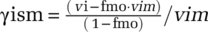 , with fmo the share of mild cases in researchers estimate of vi and vim = τa= fa·vi. Then, , with fmo the share of mild cases in researchers estimate of vi and vim = τa= fa·vi. Then, 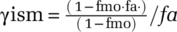 . . |
| τa | Time to Advanced Stage | 4.329 | days | Calculated/based on literature. Time between onset of symptoms and advanced stage. Consistent with estimates of hospitalization time (severe cases) (Ferguson et al., 2020). τa = fa · vi, with vi the observed viral load duration (infected); fa set to 0.667. |
| τm | Time to Recover (Mild) | 4 | days | Based on literature. Using time between onset of mild symptoms and full recovery by Ferguson et al. (2020). This parameter does not affect infectivity. |
| τr | Time to Recover (Severe) | 25* | days | Estimated.a Consistent with other studies (e.g. Ferguson et al. (2020). This parameter affects hospitalizations but not infectivity. |
| ifrs | Normal Infection Mortality Rate (severe) | 0.187 | dmnl | Estimated.a The infection fatality rate IFR is calculated as ifr = ifrs · fs.Thus, ifr = 0.0078. This is roughly consistent with other studies (e.g. Shim et al., 2020; Ferguson et al. (2020); WHO (2020b) estimating values between 1% to 1.5% but depend strongly on the share of cases exhibiting mild or no symptoms. For the component varying across countries, see Table 3. |
| fcmax | Maximum Relative Cross-Region Contact Rate | 0.0017 | dmnl | Estimated.a See further Table A.8 in the online supporting information. |
- a Estimated through cross-sectional calibration using 31 December 2019 to 15 May 2020 data on reported cases, reported deaths, recovered cases, tests performed, and on social mobility and school-closing data.
| Country | SK | GER | ITA | FRA | SWE | US |
|---|---|---|---|---|---|---|
| Virus Transmission and Clinical | ||||||
| Relative Fraction Actual Infected Cases Severea rfsd [dmnl] | 1.5* | 0.7* | 0.73 | 0.97 | 0.70 | 1 (ref) |
| Relative Infection Fatality Rate (Severe)b rifrsd [dmnl] | 0.99 | 1.22 | 1.5* | 1.394 | 1.5* | 1 (ref) |
| Time Total Cumulative Transmissions Exceed 100 τ Ed [days] | 21.9 | 21.5 | 1.6 | 9.1 | 34.5 | 5.1 |
| Social Contacts | ||||||
Reference Outbreak Level, o ref,d [dmnl] |
0.023 | 1.10 | 2.44 | 0.81 | 0.18 | 2.37 |
| Maximum Contact Reduction Fraction (Social Distancing) sdmax,d [dmnl] | 0.595 | 0.628 | 0.862 | 0.881 | 0.489 | 0.596 |
| Contact Reduction Exponent (General; Symptomatic (Relative)) βsd,d; rcrs [dmnl] with βcrs,d=rcrs ∙ βsd,d | 1.53;0.02 | 0.19;0.16 | 0.30;0* | 0.21;0* | 0.39;0.08 | 0.23;0.15 |
| Relative Efforts Needed for Full Home Confinement Ability efahcd[dmnl] | 0* | 100* | 100* | 100* | 100* | 100* |
| Testing | ||||||
| Relative Testing Capacity Growth Rate grd [dmnl] | 3* | 2.05 | 1.12 | 1.52 | 0.76 | 1.51 |
| Relative Cumulative Hospitalization for Testing Capacity Start rCHd*[dmnl] | 0.264 | 0.326 | 1.31 | 8.42 | 0.98 | 3.92 |
Desired Relative Testing Capacity  [dmnl/day] [dmnl/day] |
0.20e−3 | 0.73e−3 | 1.08e−3 | 0.32e−3 | 0.62e−3 | 0.65e−3 |
| Relative Targeted Testing Needed for Full Targeted Testing Ability efatad[dmnl] | 0.03 | 100 | 0.32 | 0.86 | 0.84 | 0.43 |
- a The fraction of cases severe is expected to vary, to some degree, across countries. Therefore, with frd = rfsd * fs, with fs listed in Table 2 and rfsd estimated using a limited range (0.7–1.5 percent) while setting d = US as reference (rfsus = 1).
- b Infection mortality rates are expected to vary, to some degree, across countries, even controlling for severity of cases. Therefore, with ifrsd = rifrsd * irfs, with irfs listed in Table 2 and rifrsd estimated using a limited range (0.7–1.5 percent) while setting d = US as reference (rirfsus = 1).
Figure 6 reports across the six countries the outbreak data (dashed lines, red), being new reported cases, new reported death rates, testing rates, and total social-contact rates (omitting new reported recoveries), and their calibrated simulated values (continuous lines, blue). Overall, the calibrated simulated data replicate a smoothed path of the noisy data.

More important, the parameter estimates generally fall within plausible ranges (see Table 2 for cross-country virus transmission and clinical parameter estimates and Table 3 for country-specific parameter estimates). To illustrate, the relative normal contacts of infected population are considerably lower than the normal contact rate of the general population (fci = 0.164). Because of adjustment delays to symptom-based behavior, this result effectively implies, controlling for infectivity, a reduction in social contacts (absent interventions) of about 67 percent. Estimation of infectivity of the infected population ii=0.635, together with those of other virus-transmission parameters, allows calculating infectious contacts and initial growth rate of the outbreak, as measured by the basic reproductive number R0. The basic reproductive number R0 is defined as the average number of secondary infections produced when one infected individual is introduced into a host population where everyone is susceptible (Dietz, 1975). Thus, a value of R0 > 1 implies active cases grow and that an epidemic can get started. The parameter estimates of the basic reproductive number of around R0 = 2.39 are close to other estimates (Read et al., 2020). On average, 4.2 percent of all cases are estimated to be severe, within the definition of the model, implying that about 1.5 percent of all cases (including mild and asymptomatic) are hospitalized. Based on the fraction severe cases fsd and the infection mortality rate for the severe cases (ifrs = 0.187), the actual estimated infection mortality rate ifrd is estimated between 0.67 percent (Germany) and 1.2 percent (South Korea), with 0.78 percent for the United States and 1.1 percent for France. This is consistent with values found in other studies ranging from 1 percent to 1.5 percent (e.g. Ferguson et al., 2020; Shim et al., 2020; WHO, 2020b). Those values likely overestimate the IFR due to the large number of cases exhibiting mild or no symptoms. The virus-transmission parameter time to recover for severe cases is estimated to be above 25 days. This value includes full recovery (or death) and is consistent with other findings (e.g. Ferguson et al., 2020).
Estimates of contact-reduction efforts highlight the considerable variation across the countries. The estimated initial responsiveness to the outbreak across countries (Table 2, Reference Outbreak Level, oref,d) suggests faster initial response by South Korea and lagged initial responses by Italy, France, and United States. For Sweden, by far the smallest country among the six, implying less heterogeneity, the combination of a lower outbreak level and higher sensitivity parameter can be explained as a population size effect. Maximum contact-reduction efforts varied considerably across the countries, and, with general-population social distancing (sdmax,d) reducing social contacts of the general population to about 49–88 percent compared to normal, with the largest effects in France and Italy and the smallest in Sweden and Germany (Table 2, maximum contact-reduction fraction (general)). The estimates suggest, however, that Germany should be viewed differently from that of Sweden in that it developed, like South Korea, targeted home-confinement ability, as can also be seen from the parameter Relative Efforts Needed for Full Home Confinement Ability efahcd, with a value close to zero. The estimates suggest that South Korea deployed other targeted approaches aggressively. This is, for example, reflected in the parameter Relative Targeted Testing Needed for Full Targeted Testing Ability, efatad, also being close to zero. In combination with total testing capacity available for such targeted testing, this parameter indicates that South Korea was able to deploy targeted testing effectively early on in the process.
Figure 7 shows more detailed results, including an out-of-sample period for a counterfactual scenario in which social-distancing policies and behavior remain in place as of 15 May 2020. The calibration against data runs from time t = 1–136 (31 December 2019 to 15 May 2020, shaded areas). The out-of-sample results run until t = 250 (5 September 2020). The left panel depicts, for a subset of countries (South Korea, United States, Sweden), simulated reported and actual cases, as well as shows the actual data on reported cases for the relevant period (t = 136). The data show a large variation in both reported and actual cases across countries. Moreover, their ratios vary considerably. Simulated actual cases on 5 September 2020 are for South Korea about 0.6 per thousand, while they are respectively 93 and 94 per thousand for Sweden and the United States. One can also infer that while in South Korea, simulated reported cases are about 37.7 percent of simulated actual cases (thus suggesting that a little under 38 percent of all cases have been detected), this value is much lower in other countries. For the United States and Sweden, these values are respectively 4.6 and 6.0 percent. Finally, the simulation shows that, whereas South Korea and also the United States (for the counterfactual assumption of ongoing lockdown as of 15 May 2020) have close to halted growth of cumulative cases, in Sweden, under a continuing but limited social-distancing policy, cases likely will considerably increase. Not shown, Germany is at 23 per thousand and France and Italy are just above 100 per thousand. Underlying these differences are the large number of mild (including asymptomatic) cases and the limited testing capacity in the beginning of the outbreak, creating a large gap between actual and reported data. However, there is more to it. The remaining graphs in Figure 7 provide additional details from the baseline simulation about the underlying dynamics. The figure highlights results for different countries to illustrate specifics relevant to different outcomes across the countries.

Figure 7 (center, top and middle) shows simulated tests performed within two comparable countries, here France and Germany, with testing differentiated by three types: (a) reactive testing of advanced-stage population exhibiting symptoms (all severe cases, Figure 4, bottom-right stock). Most of those cases involve tests performed in hospitals (tests with high priority); (b) reactive testing of early-stage populations, once they exhibit symptoms (mostly involving severe cases, Figure 4, left stocks); (c) proactive testing through field tests including through targeted approaches such as contact tracing. Simulated testing for France (center, top), suggests that initially most tests involved severe advanced-stage cases. In Germany early-stage case testing played a role much earlier. While these differences can be partly explained by differences in the early ramp-up of the testing capacity (compare the total tests performed of Germany and France), the dynamics are more complex than that.
To understand this better, consider now the case of South Korea. The baseline simulation highlights that South Korea was able to perform proactive testing even earlier than Germany. Figure 7 (center, bottom) illustrates this, showing South Korea's high case-detection fraction of not only severe but also mild cases, in contrast to those for the United States and Italy. The simulation shows that South Korea's developed contact-tracing ability (Low Relative Targeted Testing Needed for Full Targeted Testing Ability, efatad) has had a considerable impact on the positive tests. Note however that the deployment of different testing approaches is to great degree endogenous. Once a country falls behind in testing, a good part of testing capacity must be deployed to test severe cases. In this way, however, early-stage cases remain undiscovered, reducing the opportunity to identify and isolate knowable cases. In turn, those infected will maintain social contacts for longer durations, leading to greater transmission. This then leads to more cases in the long run and, through that, more testing capacity constraints. In the simulation, as in the real world, during the outbreak stage South Korea had a lower positive testing rate than other countries had during the outbreak stage. This is partly because of the higher relative testing capacity compared to other countries. However, because of their approach, a greater share of their tests involves mild cases. With positive testing rates for the mild cases being much lower than those for severe cases, during an outbreak, with constrained testing, it is difficult to move upstream toward testing earlier-stage and milder cases. Therefore, countries with testing constraints risk being pushed further and further toward reactive testing. Absent a capacity to identify positive cases in the first place, one can certainly not find others through targeted approaches. That is, a positive feedback acts to move efforts toward downstream reactive testing—away from proactively identifying, testing, and isolating upstream exposed and symptomatic populations: Once testing capacity falls behind, most cases are identified in the hospital or through severe symptoms in the late stage. (Figure A.7 shows a causal loop diagram highlighting these dynamics in further detail.) Effectiveness in targeted approaches later on thus require large testing build-up early on.
Moving to social contacts, the top-right graph shows this variable (normalized), across the whole population (thus including effects of general social distancing as well as of home confinement of suspect cases, quarantining of detected cases, etc.). The graphs show that, whereas populations within all countries reduced contacts, some did so more extensively, earlier, or faster than others. These varying responses affected the gain of the balancing feedback loop B3 in Figure 5 in different ways. For example, while South Korea was earliest to respond (low threshold), France and Italy showed the largest reduction. Sweden forms a notable exception here by having reduced contacts across all the population by just under 70 percent. The low early but subsequent rising value of South Korea and to lesser degree Germany illustrate their (successful) social-contact-reduction strategy, being aimed at isolating positive cases. Once active case counts go down, symptomatic and suspect cases reduce as well, leading, combined with some general social-distancing relaxation, to an increased average social-contact rate. Parameter estimates discussed above are consistent with this explanation. Infectious contacts together with transmission delays (incubation time—the time before symptoms begin to appear—and duration of infectivity—of the symptomatic population) determine how many people an infectious person infects during infectivity, affecting the likelihood and extent of the epidemic outbreak. The effective reproductive number R captures how changes in transmission parameters such as social contacts (as well as changes in the remaining susceptible population, negligible here) affect the growth rate of the active cases and thus of the outbreak over time. Because of the relatively high remaining social-contact rate, their current effective reproductive number is about three times that of Italy or France and close to one. Because of this, new cases, and new case detections, remain high (Figure 7, center right, showing new case detections). This graph also illustrates the fact that case detection can exhibit patterns that may differ importantly from those of actual new cases. For example, most countries exhibit a second peak in new case detections, particularly visible for Sweden. This occurs when actual new cases have peaked for the first time. If testing capacity begins to free up after hospitalizations stabilize, the detection of the (abundance of) milder cases becomes possible. Those cases previously remained undetected yielding a surge in new case detections. Nevertheless, the graph suggests that while most countries within the selection have for the most part been able to deplete the stock of undiscovered cases, for Sweden this is not the case. Figure 7 (bottom right), showing the stock of simulated undiscovered cases, illustrates this more clearly. Hence, cumulative cases keep growing (Figure 7 left, bottom). While there is uncertainty about the true ratio of actual versus reported cases, the results suggest that the share of the cumulative infections remain magnitudes below values needed for herd immunity (estimated to be about 70 percent (Ferguson et al., 2020). In this model, without interventions and testing, herd immunity builds when cumulative infections equal 83 percent of the total population). The case of Sweden suggests that controlled mitigation would be very unlikely if there are no near future opportunities to immunize the population or a multitude of subsequent outbreak waves.
The calibration analysis of Experiment 1 illustrates how timing and efforts of testing-capacity expansion and social-contact reduction interplay to affect outbreak dynamics and can explain a large share of cross-country variation in outbreak pathways.
Experiment 2: sensitivity of baseline results to behavioral responses
We next examine the effect of hypothetical changes in policy and citizen responses to the outbreak to understand better and more quantitatively how timing and efforts of testing-capacity expansion and social-contact reduction interplay to affect outbreak pathways. We begin by using the baseline for the United States as a reference from which we alter three distinct parameters and perform sensitivity analysis of simulated actual deaths directly attributable to COVID-19 to changes in: (a) the reference outbreak level for policy response (oref,US, indicated as RI); (b) maximum contact-reduction fraction through general social distancing (sdmax,US, MSD); (c) the cumulative hospitalization threshold for building testing capacity (though rCHUS*, RT); and, (d) their joint effect (all). Figure 8 (left) shows a bar graph of the simulated actual deaths (t = 250, 5 September 2020) resulting in (“high” and “low”) the values used for the parameter settings. The values roughly correspond to high (low) policy/citizen responsiveness to the outbreak as observed across different countries in the sample. (Table A.9 in the online supporting information shows the parameter values, to be compared with the baseline values in Table 3.) One can see that a more responsive government, greater effectiveness in citizens' social distancing, and earlier testing ramp up all have the effect to reduce cumulative deaths. Hence, the results suggest that each of the policy measures taken—earlier and more extensive—can considerably reduce actual deaths. Similarly, any reduced responsiveness greatly exacerbates the outbreak. Further, we see a strong interaction effect among sociobehavioral responses (see “all” vs. individual changes).

Also indicated in the bar graph are simulated actual (thick line segments) and reported cases (thin line segments) compared to the baseline (dashed line). While actual cases correlate highly with the actual deaths, reported cases are particularly less responsive in the test (RT) scenario because high (low) responsiveness implies that higher (lower) testing capacity makes up for the increased (reduced) actual cases of which more (fewer) are captured. Further, increased actual cases creates precisely those problems that make it hard to keep up with testing. This observation is important because reported cases are main drivers for decisions and citizen responses. This itself contributes to the strong effects we observe in the actual cases. While it is problematic to use responsiveness to reported deaths as an indicator (with lags between infection and death being three to four weeks), the sensitivity analysis shows the risk of underestimating the effects of too little action, when driven by reported cases (especially when relative reported cases are low).
The sensitivity to timing and extensiveness of interventions has not only implications for long-term indicators such as cumulative deaths, but also affects transitory variable, with an implication on the health system. Hospitalizations accumulate with long lags between transmission, onset, and appearance of advanced-stage symptoms. Hospitalizations decline after recovery or deaths, which itself can last several weeks. Together, this implies strong amplification of peak hospitalizations (Figure 8, top right, with response to same policy parameter changes). The scale is comparable with that for cumulative cases (red bars in the figure). However, while the day-to-day changes in cumulative deaths or cumulative cases are relatively moderate (not shown), for a transitory state like hospitalization, a similar amplification can build up within 30 days, with dramatic consequences for manageability of the health system.
Interaction effects between behavioral responses to the outbreak require further examination. Figure 9 (left) shows the joint sensitivity of simulated actual cumulative deaths (ADUS, per thousand people) to changes in reference outbreak level for policy response (RI) and the threshold for testing capacity the cumulative hospitalization for testing growth rate (RT). Higher responsiveness to interventions (RI) is toward the left while higher responsiveness to testing (RT) is toward the bottom (Table A.9 in the online supporting information indicates the parameter values). In the graph, a number of reference points are indicated with values for ADUS (darker colors indicate higher number of deaths), including those corresponding with the baseline (ADUS = 0.80) and the low/high univariate changes in Figure 8. Also indicated are simulated initiation times of interventions and of testing build-up for the baseline case ( and
and  ) as a result of the responsiveness thresholds, with differential values, compared to the baseline, for the other reference points. The results highlight the strong sensitivity to the timing of the build-up of testing capacity (top to bottom), corroborating the conclusions inferred from the different baseline results in Figure 7 (center graphs). Additionally, however, while a moderate higher/lower response has the effect of reducing (lighter colors)/increasing (darker colors) cumulative deaths, their joint effect amplifies these impacts. Thus, for example, policies that stimulate social-contact-reduction efforts are greatly enhanced when policymakers and citizen have a more accurate perception of the extent of the outbreak. To see this effect, compare the two (red) dots indicating low responsiveness of either RI or RT (low RI, ADUS = 1.06 and low RT, ADUS=1.10) with the (white) dot indicating their joint effect (low RI & TI, ADUS = 1.44). Note further that the delay in the intervention response compared to the baseline is larger for the joint effect of RI and RT than for RI alone
  versus
  . Similarly, increasing responsiveness of both levers (toward high RI and high RT) shows strong synergistic effects. While at this point care must be taken in taking too much confidence in specific parameters and outcomes, quantitatively the results indicate that higher (lower) responsiveness in either testing capacity build-up or of social distancing that result in accelerated (delayed) action by a week could, in the United States, reduce (increase) cumulative deaths by about 50 percent (about 0.5 deaths per thousand people). Even greater (lesser) responsiveness in testing and intervention could further reduce (increase) deaths.

These quantitative and even qualitative insights do not necessarily hold for other situations. In particular, high responsiveness across multiple interventions early on may reduce sensitivity to changes in a single intervention. Figure 9 (right) highlights this, showing, now for South Korea, the effect of the reference outbreak level for policy response (RI) on actual cumulative deaths, but jointly with the effectiveness of one of the targeted approaches—the Ability to Identify Associated Cases for Home Confinement (SUS). Higher responsiveness is again toward the left for RI but is toward the top for SUS; the color coding is rescaled to match much lower deaths for South Korea. The calibrated baseline setting and result are indicated in the top right. The sensitivity analysis for RI in the case of South Korea shows that, while weaker responses in RI have important relative effects on deaths, they do not alter much the absolute scale of the epidemic impact. This is so because South Korea had a number of policies in place that enabled it to respond effectively beyond rapid response and home confinement of suspect cases. This includes not only extensive testing (Figure 1), but also a focus on mild cases (Figure 7 (center bottom), among others. Interestingly the results of Figure 9 (right) suggests that, during the very early stages, interaction of just one targeted approach variable, SUS, is modest to weak (but nonzero; A similar sensitivity test for United States and most other countries in the set shows virtually zero responsiveness).
Together the results of Experiment 2 highlight how the extraordinary measures taken in some of the early outbreak countries were critical to control the outbreak. In particular, the combination of extensive and effective testing and finding ways to reduce general social contacts are critical. Combining multiple interventions creates slack in testing capacity, as was the case for South Korea. The slack in testing capacity frees up resources for more proactive efforts. Thus, by taking these multiple actions timely and aggressively, one achieves important redundancy in response to the outbreak. The results also suggested that targeted approaches, while importantly complementing other approaches, are ineffective when testing capacity is relatively low and cases are high and growing. We will see the vital role of targeted approaches during postpeak stages in helping build up a stock of potentially identifiable existing and at-risk cases. The analysis further illustrates that, once a country falls behind, just improving testing along with detected cases is not sufficient—such as has been the case for the United States.
Experiment 3: managing deconfinement
The following experiment focuses on the challenge of managing deconfinement. Because confinement involves high social and economic costs, there is pressure to reduce this at some point after (or even before) active cases begin to reduce. But how much can a country deconfine? What system needs to be in place in a country to be prepared for deconfinement? Specifically, how do targeted interventions and testing help the deconfinement? Illustrating one aspect of this challenge, we define deconfinement here as the (partial) reduction of social distancing for the general population. To illustrate some of the key tensions, we perform an analysis within a stylized context, closely related to the baseline. Consider a region of 16 million people (the approximate size of a metropole like New York or Paris, of the hard-hit region of Northern Italy, or of a country like the Netherlands) with starting-point characteristics similar to the average of the countries we analyzed before in the baseline (see again Table A.9 in the online supporting information for the relevant parameter settings). I then introduce a COVID-19 outbreak with 100 undetected infections. Next, at deconfinement time τdc=10, counting from the first time reported new cases begin to decline, policymakers begin to reduce a fraction fdc ∈ [0, 1] of the social distancing that has endogenously emerged. A value of fdc = 0 indicates no deconfinement (similar to our counterfactual baseline scenario) while fdc = 1 means full deconfinement. Deconfinement is ramped up to the level indicated by fdc during a period τdd= 60 days after which the deconfined state remains at that level. Deconfinement is restricted to contact-reduction policies related to undetected and nonsuspect cases only—so, for example, quarantining of detected cases and home confinement of suspect cases (see Figures 2, 5) remain in place. We perform the experiments, varying a number of parameters, with particular focus on the role of targeted approaches during deconfinement.
Figure 10 shows, as before, a number of graphs of simulated cumulative actual deaths AD (now at time = 500, to assure stabilized results), here as a function of the ability to identify associated suspect cases for home confinement fahc (SUS, horizontal axes), which we also used in the previous experiment (Figure 9), and the deconfinement fraction (FDC, vertical axes). Note that the percentage of general social contact restored given a deconfinement fraction depends on the maximum social distancing sdmax pre-deconfinement. Here we use sdmax = 0.65, comparable to an average country within the calibrated set. Therefore, in this case, 50 percent deconfinement (FDC = 0.5) restores up to 67.5 percent of social contacts. To restore social contacts to 80 percent requires FDC = 0.69. The graph indicates these two values for reference. We plot these results for low versus high contact tracing ability (CT: left versus right graphs) and for low versus high relative initial experience with targeted interventions and testing (ETA: top versus bottom). Table A.9 in the online supporting information lists again all the parameters adjusted for the experiment. Each graph shows two reference points, both at zero deconfinement efforts (FDC = 0), indicating AD for respectively zero and high ability to identify suspect cases for home confinement. The graphs highlight as a single gray shade any parameter regions with actual deaths exceeding two per thousand (see areas with “AD>2”). This cutoff value is chosen, being about twice the largest number of deaths absent deconfinement (see values indicated in the bottom left of each graph, FDC = 0 and SUS = 0). Values AD=2 are market according to the color code on the right.

The graphs show, first, a very strong nonlinear response to the deconfinement fraction. The graphs nicely highlight that for each graph, for sufficiently low deconfinement (low FDC) cumulative deaths remain very close to the unconfined scenarios (FDC = 0), well-below 1 per thousand. However, beyond some critical value of FDC, deaths move above 2 per thousand. Simply put, above some threshold, the reproduction number becomes larger than one (R > 1). Safely avoiding resurgence risk requires staying well below this threshold. The different figures show what conditions and measures and combination help increase this threshold. Moving across the four graphs, one can see that the key lies in a strong ability to identify and home-confine suspect cases can help increase the level of deconfinement. The contrasts between the bottom graphs (high initial experience with targeted approaches) versus the top graphs (low initial experience) show that having abilities to identify and isolate suspect cases needs to be in place before deconfinement starts. Once deconfinement starts, active cases decline at lower rate than otherwise, or may grow again, or, and with that, resources to perform targeted approaches as well as general testing itself risk becoming overloaded. Therefore, we may expect that countries such as South Korea and Germany will be able to manage deconfinement more effectively than most other countries.
Second, comparing the left versus right graphs highlights positive interaction between contact-tracing ability (CT) and home isolation of suspect cases (SUS). By itself, contact tracing may not have a large impact on deconfinement outcomes because contact tracing does not directly alter the reproductive number much. However, contact tracing does enable a more effective isolation of a number of potential positive cases and in this way strengthens the effect of suspect case identification. To illustrate this, the benefits of CT are much greater for larger than for smaller SUS.
The deconfinement analysis so far suggests the vital importance of capacity for targeted approaches (general testing capacity, effective contact tracing and testing, extensive and effective confinement policies for suspect cases). A next important question is how do social-distancing policies prior to deconfinement affect the feasible extent of deconfinement? One can get insights into this by comparing results for values with different pre-deconfinement maximum social distancing sdmax levels (MSD). (Note again, for example, that for Sweden sdmax = 0.49, while for France sdmax=0.88, Table 3.) Figure A.8 in the online supporting information shows such a comparison using sdmax = 0.5. The results show that for well-developed targeted approaches, the threshold for a renewed outbreak is lower for countries with lower initial MSD. This is presumably the case because the larger number of active cases upon deconfinement make it harder to keep down the suspected case pool. Thus, low MSD countries face larger deconfinement risks than high MSD countries. So, a country like Sweden will face larger deconfinement risks than a country like France or Italy, assuming identical deconfinement time and abilities for targeted intervention and testing.
In summary, Experiment 3 shows that deconfinement requires countries to be ready. Readiness means low active cases, high testing capacity available, including for mild cases, and having capacity for targeted approaches (suspect case identification, for example, through contact tracing and effective suspect case isolation). More quantitatively, absent strong capabilities for targeted approaches that allow in-the-field case detection and suspect case isolation, deconfinement of 50 percent, so to restore postpeak social-contact rates to about 60–70 percent of prepandemic levels, leads very likely to renewed outbreaks (Figure 10, top). Staying well below these values is of vital importance. Targeted approaches may allow deconfinement to increase by 10–30 percent due to abilities in early new case detection and actual and suspect case isolation. Given the large sensitivities, citizen compliance, so to maintain the degree of deconfinement and assure effective suspect case isolation, is critical.
Experiment 4: managing resurgence
Next, we highlight the challenge of managing resurgence. Given that building up herd immunity during a first wave is not a feasible strategy and because of the present absence of vaccines, it is highly likely that additional outbreak waves will occur in the near future (Ferguson et al., 2020; Kissler et al., 2020a). Contrasting a first wave, during resurgence, reasonable testing capacity will likely be available. Hence, generally, in contrast to first-wave outbreak responses, for postpeak strategies, proactive testing approaches are generally feasible. We use the same setup as for Experiment 3. However, to allow for resurgence, we now let policy makers and citizens respond to the reported active (instead of cumulative) cases. Hence, once reported active cases go down, citizens and policymakers begin to relax their social contact reductions. As a result new cases gradually grow again. Also different from the deconfinement scenarios, we now allow society to return to contact-reduction strategies in response to a resurgence. Depending on response sensitivities and behavioral and virus-transmission delays, a cyclical pattern of active cases results. Figure 11 shows simulations using synthetic data of a representative case. (See Table A.9 in the online supporting information for all parameters differing from the baseline.) The base case (continuous line, blue) does not include any targeted approach. The simulated actual active cases (top left) show the cyclical pattern. At some point, the virus outbreak appears to be receding, as actual (and reported) cases go down considerably. As social distancing rebuilds (center), the virus can transmit again easier among the population allowing a second wave to commence, and so forth. Cumulative deaths (bottom left) keep rising considerably with each wave. While, naturally, susceptible cases decline (inset), the decline is not sufficient to strongly reduce the reproductive number, let alone build herd immunity. The cyclical patterns of social contacts and hospitalizations highlight the high societal costs associated with the base case.

In this case, proactive testing may be expected to play a critical part of effective responses to endogenous resurgence patterns because the society will also respond by reducing social contacts. Having an ability to identify positive cases could help in this responsiveness. To understand the impact of targeted approaches, we now vary targeted testing effectiveness, measured by the clustering parameter rκta. The strongest effectiveness corresponds with rκta=50. First notice that all scenarios respond similarly to the first wave, irrespective of proactive testing effectiveness, highlighting that constrained testing capacity initially limits targeted testing. (Further, this first wave is identical to what it would have been in case of a population responding to cumulative cases.)
While the amplitude of the oscillatory pattern persists in the base case, proactive testing effectiveness (higher rκta) is effective in dampening the oscillation amplitude of new cases (Figure 12, top left). The rapid detection of new cases takes an important share of the newly introduced symptomatic population out of contact risk (Figure 12, center), and the symptomatic population remains at a relatively low level. The policy is very effective in not only reducing oscillations and overall emergence of new cases but also, in this case, suppresses oscillations of social distancing and, for high-contact tracing, stabilizes this at around 60 percent. Scenarios with lower social-distancing sensitivity (not shown here) can more rapidly stabilize social contacts, at higher levels of about 70 percent of normal contacts. Consequences for society are large as can be seen in reduced average and peak hospitalizations (Figure 12, bottom right). While more work is required to analyze resurgence dynamics, this analysis suggests that reduction in responsiveness to internally produced resurgence is, under the circumstances, more important. This is so because this stability helps the effectiveness of targeted approaches that benefit from stable use of testing and other resources.

Experiment 5: dynamics of vulnerable population segments
Symptom severity, hospitalization, and infection fatality rates differ considerably across age groups, with the older population being disproportionally vulnerable to the impact of the virus (Kuchler et al., 2020). In a final analysis, we use the model segmentation to help better understand how these differences affect the different population groups as well as the overall outbreak dynamics. To illustrate the value of analyzing this in more depth, we focus in particular on explaining the role of different social interactions across these segments in different countries in explaining the outbreak patterns. We perform an analysis in the same stylized way as the previous experiment. We again use a stylized region of 32 million people, but now we divide the population equally over two segments, varying only the fraction of cases severe (fsd) between them. The segment with higher (lower) fraction of cases severe represents the more (less) vulnerable population segment (for example, “older” versus “younger” populations, though note that the distinction can also proxy other stratifying variables such as income or race). We control the difference in fraction of cases severe between the segments by varying the relative fraction of cases severe for segment 2 (rfs2), relative to that for segment 1, holding the average infection fatality rate constant across the segments. Testing capacity grows as before, with an initiation threshold of 100 hospitalized cases. At time 0, we introduce again a COVID-19 outbreak with 200 undetected infections, but only within the less vulnerable population segment. (Table A.9 in the online supporting information shows parameter details.)
Figure 12 shows the results. The graphs vary horizontally the relative fraction of cases severe for segment rfs2. A value of one indicates that the fraction of cases severe (and therefore the infection fatality rate) is identical across the two segments. Smaller values of rfs2 (moving to the left) signify increasing heterogeneity, with the presence of an increasingly vulnerable population segment. The left graph shows the actual cumulative cases (left vertical axis, per capita)) and actual cumulative deaths (right vertical axis, per thousand people (ptp)) as a share of the population. Results are shown for two different relative contact rates between the segments ( , controlling for total contact rates within the population. Continuous (dashed) lines have high (low) intersegment contacts. The graph shows a number of interesting insights about how cases and deaths develop as we vary these two parameters. In particular, when case fatality is uneven, actual cases increase (left graph). This is so because low vulnerability implies on average milder symptoms and, because of that, lower detection. With low reporting there is little policy response, and infections can easily spread among the less vulnerable populations. A relevant but not unrealistic starting condition in this analysis is that the outbreak initiated among the young population. For example, in regions like New York City, it appears that in the socially active younger population (with mostly mild symptoms), the virus has spread rapidly while remaining fairly undetected for a while.
The right graph shows the relative cumulative deaths in three different ways: total versus reported, total versus actual cases, and the share of vulnerable population to the total. (For reference, one can see that this share reaches to 50 percent at high intersegment contacts, when rfs2 = 1, thus fs1 = fs2.) The results further show that the worst case in terms of absolute fatalities, high variation in case fatality, and relatively high contacts between the population segments, disproportionally affects the vulnerable population (dashed line, top right). This is so because after the virus has spread among those who are less vulnerable, it can easily spread to the vulnerable population segment, at which point it is uncontrollable. It is the latter that may have been playing a part in Italy, with relative contacts across generations generally being larger than in many other countries.
While only a synthetic analysis, these results on stratified vulnerability may partially explain the large variation in reported death fractions (case fatality fraction, CFR) across countries or why the reported CFR in some countries seems low for a while, only to go up later, and counters the expectation as recoveries and death accumulate. These insights also imply that policy recommendations may vary depending on the demographic makeup. For example, when relaxing general confinement policies, or when managing resurgence, should populations that are deemed more vulnerable remain (longer) isolated at home? Based on the insights here, that may be a feasible direction, provided that mild cases can be detected and isolated.
Discussion
This article developed a behavioral infectious-disease model capturing how virus-transmission dynamics and policy and citizen responses interact to shape the course of an epidemic virus outbreak. Applicable to the full epidemic cycle including deconfinement and resurgence, the policy model allows exploring the impact of individual and joint policy interventions. Most essentially, the results can not only explain the large variation in outbreak paths between countries but also provide guidance for addressing postpeak strategies and the conditions under which these work.
To study implications of different interventions and testing strategies, the model incorporates some key behavioral aspects and disaggregates critical constructs. Central to the model are not only virus-transmission dynamics, following SEIR-based epidemic modeling traditions, but also explicit formulations of policymakers ramping up testing, reporting, and interventions in response to the outbreak and populations altering their social contacts, with potentially imperfect compliance. The model differentiates cases with mild symptoms (including asymptomatic ones) from those with severe symptoms, captures reactive as well as proactive testing, and represents different social-contact-reduction interventions for general, suspected, and detected populations (including social distancing, home confinement, and quarantining). Finally, the model allows representing heterogeneity across sociodemographic and geographical population segments, including interactions among them. Together the key metrics—over-time reported and actual positive cases and deaths, hospitalizations, and social-contact reductions—allow not only studying outbreak dynamics (first wave, deconfinement, and resurgence) but also help consider societal implications—health system overload, recurrent social distancing—resulting from the different scenarios. Thus, the model can be used to evaluate the broader impact of diverse public health control measures, to consider interactions with testing and reporting and citizen response.
Using the model to explore both current questions about managing the COVID-19 outbreak response and postpeak strategies yielded important policy insights specific to the current pandemic as well as relevant for policy and to infectious disease modeling in general. An explanatory analysis demonstrated the workings of interplay among distinct interventions and/or citizen behavior. For example, efficacious interventions not only require willingness to implement multiple ways of social-contact reduction but also early testing capacity. Limited case testing delays implementation of any social-distancing interventions rendering them considerably less effective. Calibration of the ongoing COVID-19 outbreak to data from six countries suggest that such interplay among timing and efforts of testing-capacity expansion and social-contact reduction can explain a large share of cross-country variation in outbreak pathways. Quantitatively, the strong transmission feedback combined with dynamics toward reactive approaches implies that, in the case of the United States, a one-week delay in testing/intervention build-up can be as costly as 25–50 percent additional cumulative deaths. Second, deconfinement analysis suggests that societies will have to find ways to effectively reduce social contacts of asymptomatic population to about 60–70 percent of prepandemic levels as long as no pharmaceutical solutions are available at scale. A country's preparedness for deconfinement can significantly reduce risks of renewed large-scale outbreaks. In particular, the presence of effective and extensive targeted testing and intervention approaches (contact tracing and testing, broader suspect case isolation, surveillance, and isolated case compliance) are vital to reduce resurgence risks during and after deconfinement.
What are some of the implications of these results about deconfinement and resurgence policies? First, deconfinement of, say, 50 percent of prepandemic social-contact levels involves a major societal challenge, especially within a reality of heterogeneous behaviors and partial compliance. Clearly, health experts must define and communicate rules where and to what extent vital social-distancing practices such as physical distancing, mask wearing, and personal sanitation should be implemented. But beyond those rules, absent guarantees of near-term vaccination or other forms of long-lasting mass immunity, societal innovation for sustainable social distancing is critical. Second, effectiveness of targeted approaches also requires at the moment of deconfinement the presence of low active cases, high available testing capacity, high citizen willingness to be tested (including from those with mild cases), and rapid test results. Further, slowing the pace of deconfinement, while not affecting the reproductive number in the long run, may make it easier to build targeted capacity, to learn, to monitor, and to respond to local resurgent outbreaks and to impose temporary regional lock-down if needed. Third, implementing targeted approaches may imply partial reliance on contact-tracing apps. It is essential that such apps are developed without compromising privacy safeguarding. The effectiveness of such apps and safety further requires coordination across countries with large traffic flows. The need for targeted approaches also suggests, beyond the apps, a strong opportunity to put more responsibility with citizens within communities and to support their capability development and awareness for suspect case identification and isolation.
The final analysis, with population disaggregation into segments of higher versus lower vulnerability, demonstrates not only how different population groups can be differently affected by the outbreak but also illustrates that such heterogeneity itself can affect (worsen) the overall outbreak dynamics. Together, the analysis shows the nature of nonlinear and complex, multifeedback systems being resistant to change. Significantly altering the pathway of a focal variable within the system requires a mix of interventions to address different positive feedback loops and delays within the system.
In terms of the model itself, this model adds to the existing body of epidemic policy models by combining a range of policy and testing instruments and behavioral aspects particularly critical to infectious diseases that are characterized by high reproductive numbers, high fatality, but generally low severity of cases. Further, while calibration across a variation of countries with different policies demonstrates the model's robustness for the case of COVID-19, the model is flexible in that it can be applied to other infectious disease contexts. While the analyses demonstrate that fundamental insights can be derived with a relatively aggregate model, additional subsequent empirical analysis on country- or region-level analysis, involving varying epidemic pathways and policies, can provide further insight into the specific parameter values related to both virus transmission and social behavior. The detailed documentation and model availability facilitate replicating and expanding the model and analysis for similar and other contexts.
The model and analyses suffer from usual limitations as well as from those particular to the case of an emergent outbreak. First, the relatively aggregate representation of population segments implies that some important dynamics may have been missed. For example, the emergence of superspreader events could be important (Lau et al., 2017). While the model allows an analysis of targeted approaches, it is currently not adjusted for examining such forms of heterogeneity. Given the relative aggregation in the current analysis, the model likely underestimates the value of targeted approaches. The model in its present form also leaves out important structural elements, such as endogenous infections and fatality within the health-providing system (Fiddaman, 2020).
The present analyses and limitations listed here suggest multiple opportunities for further work. For example, in terms of analysis, given that the pandemic has reached the peak of a first outbreak wave for many countries, subsequent analysis should focus more on managing the transition toward deconfinement and resurgence waves. The experiments show that the model is well-suited for such analysis. The full model also has a tentative substructure that allows the implementation and roll out of (potentially imperfect or slow) vaccinations, as well as the role of immunity loss rate. While switched off for the purpose of this article, understanding these dynamics in combination with resurgence dynamics will soon be important (Kissler et al. 2020a). For example, to what extent does the promise of future vaccine availability with nevertheless uncertain roll-out times negatively affectthe stringency of and compliance to existing interventions?
Second, there is a need to focus on the question of “what are fruitful confidence building efforts for dynamically complex but still developing cases like this one?” Within such contexts, policy decisions as well as supporting modeling efforts take place under large and evolving uncertainty. Given this, the purpose of the analysis here has not been to just generate specific policy findings but also to develop a broad-boundary model that can facilitate a more grounded understanding of the pre- and postpeak outbreak dynamics. In this article, the analytical strategy for gaining confidence in this understanding focused on: (a) a calibration with plausible estimates; (b) a detailed dynamic analysis of an out-of-sample counterfactual baseline; (c) comparing and interpreting different policy interventions using this baseline; and, (d) documentation of the model and analysis results that allow replication and further interrogation and exploration.
Additional efforts that help build confidence in the findings can of course include additional confidence interval analysis. But, when performed in isolation, any inferences must be drawn with great care, because much uncertainty remains undetected by confidence intervals. For example, Experiment 5 highlights that sociodemographic heterogeneity can strongly affect diffusion dynamics. Such dynamics are particularly relevant for cross-country comparison and for analysis within countries having larger geographic areas and populations, such as the United States. Similarly, any forward-looking analysis may easily miss future policy and citizen behaviors differing from those simulated here because of behavioral, technological, or administrative adaptations. Finally, unavoidable choices by the researcher about calibration weights across multiple estimated data series affect confidence-bound estimates.
As a result, confidence-building efforts within such dynamically complex and developing contexts must also consider how variation in structural assumptions, forward-looking scenario choices, and time-series analysis within the calibration process individually and jointly affect the ability to draw confidence-related inferences. As a start, this requires models that generate explainable dynamics and behaviors. Underlying models therefore need to be not only robust but also transparent about the mechanisms and the behaviors as modeled—so they can be challenged and built upon (Barton et al., 2020).
The need for rapid policy responses combined with on-the-ground learning of expert decision-makers, a turbulent and dynamic environment, limited and emerging data, requires a process that can make those models more rapidly accessible to those experts as policy tools. One component of such a process could be a formalized expedited review process guaranteeing usual rigor. While such processes exist, they are less accessible for broader-boundary models. Second, as with climate action, much of the intervention success depends on broad support and involvement from many actors outside directly involved experts—local policymakers who have no direct access to the experts, volunteers with efforts within communities, citizens who comply, media that communicate, etc. Therefore, making the models accessible as web-based management flight simulators is critical as well (Rooney-Varga et al., 2020). The operational details and behavioral aspects of this model also allow developing such an interactive policy tool.10 Finally, to effectively inform policymaking within this evolving context, such a process needs to yield robust tools that are updatable while remaining grounded in ongoing empirics.
References
- 1 Therefore, the model can also be used to explore how the dynamics change depending on assumptions related to different infectious diseases, such as SARS, HIV, and H1N1 and H5N1, Influenza, and Ebola.
- 2 Most countries that responded well have had previous experience with the SARS epidemic (2002–2003).
- 3 Reported cases and testing data were retrieved from Ourworldindata.org (Roser et al., 2020). The mobility metric combines data on intensity of walking, driving, and public transport use (retrieved from the Apple Maps Mobility Trends Reports, Apple, 2020), each equally weighted. Values are relative to the reference value of 18 January 2020. Data on school closings (retrieved from Unesco, 2020) are on a relative scale from 1 (all schools open) to 0 (all schools closed).
- 4 This is a simplified representation of the virus-transmission rate. In the model, the stocks of exposed and symptomatic populations are each disaggregated into different stocks with different contact rates. For example, part of either population segment may be quarantined or home confined (discussed below).
- 5 An alternative to cumulative reported data as inputs to the perceived outbreak level would be recent deaths and active cases, for capturing, somewhat simplistically, fully endogenous easing of social-contact reductions as the perceived severity of the outbreak declines. Indeed, experiment 4 below, examining resurgence dynamics, uses these alternative inputs. However, for all the other analyses in this article cumulative reported data serve as input for the perceived outbreak level to examine the effect of deconfinement interventions in more controlled ways.
- 6 Purely hierarchy-based prioritization is a useful but somewhat crude simplification of reality. In the model, the parameter “sensitivity for testing prioritization,” βt, moderates the propensity to allocate testing capacity according to relative desired testing rates. βt=0 implies tests are performed according to capacity needs (and hence, potentially a tendency toward proactive testing). Higher values imply stricter allocation according to priority (implying a tendency toward reactive testing). The simulations below run with the extreme case of fully hierarchical testing-capacity allocation.
- 7 Simulated actual deaths is not only a policy variable of central interest, the variable is also fairly robust against structural assumption changes. This contrasts in particular “simulated actual cases” which tend to be sensitive to varying assumptions. This is so because it directly depends on the hard to observe mild/asymptomatic cases (which do not cause deaths).
- 8 The online supporting information includes a folder with all files and data necessary for replicating the experiments using the provided Vensim model. Appendix A.II describes the estimation procedure and data in more detail. Appendix A.V includes the instructions for replicating the experiments.
- 10 As illustration, a simplified version of the model analyzed and provided in this article is available as a free web-based management flight simulator (Struben, 2020).