Computational Improvements to the Kernel -Means Clustering Algorithm
Funding: This work was supported by National Institute of Food and Agriculture.
ABSTRACT
Kernel k-means (kk-means) extends the standard k-means clustering method to identify generally shaped clusters by employing the k-means algorithm in a higher-dimensional space. Current implementations of kk-means are rather naive. We present simplifications that reduce calculations, performing only those that are absolutely necessary, therefore improving the overall algorithm's run time. We also present a sampling-based clustering and classification strategy for employing kk-means clustering for large datasets. Results on 13 data sets illustrate the computational benefits of our new algorithm. Our sampling-based strategy is also applied to investigate the use of -means in the color quantization of images in human perception-based colorspaces.
Abbreviations
-
- AAC
-
- alternating assignment and centering
-
- ARI
-
- adjusted rand index
-
- kk-means
-
- kernel k-means
-
- MATR
-
- MAx-TRace
-
- MKNN
-
- mean k-nearest neighbors
-
- OT
-
- optimal transfer
-
- OTQT
-
- Optimal transfer and quick transfer
-
- QT
-
- quick transfer
-
- SCAC
-
- sampling-based clustering and classification
-
- SDSS
-
- Sloan Digital Sky Survey
-
- SRSWOR
-
- simple random sampling without replacement
-
- VIF
-
- visual information fidelity
-
- WSS
-
- within-sums-of-squares
1 Introduction
Cluster analysis [1-4] partitions observations into homogeneous groups without label information. There are many clustering applications [5-9] and methods [10-16], of which the most commonly-used is the model-agnostic -means algorithm [17-19] that partitions observations into a given number () of groups by locally minimizing the WSS. The preference, by design here, is for homogeneous spherical clusters, even though attempts [20-23] have been made to address this limitation. Similarly, the -means algorithm [24, 25] performs -means-type operations after nonlinear mapping of the data onto a higher-dimensional space, but is slow on larger datasets.
This paper proposes three sets of computational improvements to the -means algorithm. We recognize that current -means implementations adapt [17]'s -means algorithm that, upon starting with initial cluster centers in the transformed space, assigns each transformed observation to the cluster with the closest center, and then updates the centers at the conclusion of the cycle. Our first improvement borrows ideas from [26]'s -means algorithm and simply updates cluster centers with every observation reassignment. Our second improvement forms the crux of our contributions and simplifies and reduces computations by utilizing an “optimal transfer” (OT) stage and a more heuristic “quick transfer” (QT) stage, as also done [27, 28] for -means and -modes algorithms [12]. Indeed, OT steps are proved to improve solutions. Finally, we explore a computationally feasible clustering and classification framework for -means on large datasets.
This paper has four more sections. Section 2 details the methodological improvements mentioned above. Section 3 evaluates performance on some common synthetic and real datasets. The modification for use with large datasets is employed to study the use of -means for image color quantization in human perception-based colorspaces. This article concludes with a discussion. A supplement, with sections, tables, and figures prefixed by “S” is available, as is a R [29] package kkmeans that implements our methods.
2 Methodology
2.1 Background and Preliminaries
Consider a dataset with -variate observations . The usual -means setting partitions into disjoint sets by minimizing the WSS , where . Kernel methods generalize this framework.
These kernels have user-specified parameters that are estimated, as discussed in Section 2.2.3.3. This paper uses the Gaussian kernel, but our methods apply to other kernels.
Current implementations of -means simply mimic [17]'s -means algorithm that naively assigns each observation to its closest current centroid, updating the centroids only at the end of all the assignments. We suggest improvements to this approach in the remainder of this section.
2.2 Efficient -Means Algorithms
2.2.1 Alternating Assignment and Clustering (AAC)
Our first improvement updates the cluster centers with every reassignment of an observation to a centroid. Indeed, [26]'s -means algorithm fits the AAC framework, and we shall see that this seemingly simple fix improves both accuracy and running time of the -means algorithm.
2.2.2 Optimal Transfer and Quick Transfer (OTQT)
- For each observation , find and store its closest and second closest cluster centers, and , and assign to .
- Initially, all clusters are in the live set .
-
Optimal transfer. Consider the cluster . Then only if was updated in the last QT stage or if it was updated in any of the last OT steps.
-
Let . For , find
()If no reallocation is necessary and . Otherwise, transfer to and set . Clusters and are now in the live set .
- For , proceed as in Step 3a but with in (3) minimized only over .
-
- Stop if is empty. Otherwise, continue to Step 5.
- Quick transfer. Let and . If then skip to . Otherwise, transfer to and set if
- If no changes occurred in the last QT steps, go to Step 3 otherwise go to Step 5.
Claim 1.Let be the center of in feature space after initialization. The -means algorithm using only OT steps with distinct observations and distinct initial centers has the following properties:
- Each pass through the dataset never increases .
- The resulting partition set has no empty clusters.
- Each pass through the dataset keeps the centers distinct.
- If there is no that can reduce the objective function by transferring to a different cluster, the algorithm will terminate. Additionally, an observation will only be transferred to a different cluster if the objective function decreases, proving Part 1.
- Suppose at the beginning of the OT stage. Then reassigning any to will reduce , and so will pull in at least one of the s. Alternatively, suppose a cluster is made empty during the OT stage. Then, the algorithm will iterate due to an observation being transferred, and a point will be assigned to the empty cluster. So, Part 2 holds.
- Suppose upon entering the OT stage, . Then, since each point is distinct, there exists a point such that . WLOG let . Then, since and , the reallocation condition in the OT algorithm is met and will be transferred to .□
The OT steps can be implemented in parallel to further speed up computations. Further, we see the QT steps to substantially improve experimental performance, but as with -means [32] or -modes [12], these gains have not been possible to prove theoretically.
2.2.3 Additional Implementation Aspects
We address a few issues that arise while implementing our algorithms.
2.2.3.1 Initialization
As with -means [33], initialization of -means algorithms impacts clustering performance. A simple approach is to use SRSWOR to choose random observations in feature space. This method was not outperformed by our -means++ approach (Section S1.1) that extends [34]'s -means++ algorithm. Our initializer is stochastic, so we run our algorithm from many initializers and choose the result with the lowest terminating of (1).
2.2.3.2 Storing Distances
For the Gaussian kernel, is constant and can be ignored in calculations. Additionally, and can be stored for each . If has been transferred or if either or have changed since the last time was visited, these values must be recomputed. This recomputation requires computations of and can be expensive, so if computer memory permits, it is better to store the Gram matrix for the dataset and thus reduce the number of computations. Such an approach can also be adopted for our AAC algorithm, since the centers are updated whenever an observation moves to a new cluster.
2.2.3.3 Parameter Selection for the Gaussian Kernel
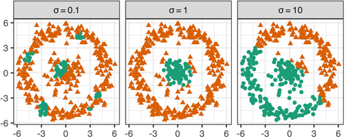
The Gaussian kernel needs a choice for the bandwidth parameter . Figure 1 illustrates the effect of on -means clustering of the Bullseye dataset [21, 22]. We see that smaller s produce fragmented groups in Euclidean space, while larger values produce more compact clusters. We now discuss some methods for choosing . Luxburg [23] suggested estimating using the mean squared distance of each observation to its -nearest neighbors (MKNN). Ordozgoiti [35] provided a hierarchical search method that requires storing the full Gram matrix, and is impractical for larger datasets. The MAx-TRace (MATR) algorithm [36] performs a grid search on the possible values of . The algorithm needs a similarity matrix of the data: we choose by using , with preliminarily estimated by MKNN, with . Section S1.2 shows our MATR implementation to outperform MKNN. The method also extends to non-Gaussian kernels, and so we use it hence.
2.3 The -Means Algorithm for Large Datasets
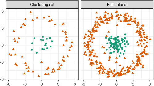
Even with our improvements, our -means algorithms can still be slow for large datasets. This is because beyond the in-place calculations of the Gram matrix needed for large , the kernel function has to be computed for each observation in each cluster, even before any feature space calculations. We propose a sampling-based clustering-and-classification (SCAC) strategy for large datasets. Specifically, we randomly split the original data into a set used for clustering, and the remainder used for classification. We cluster using -means to obtain a partition of clusters . Then the observations in are assigned to their closest cluster in according to (2). For illustration, Figure 2 displays the use of our SCAC strategy for the bullseye dataset. aset of 200 observations. While our -means algorithms can be easily applied to this dataset (and is done in Section 3), our illustration using only 20% of the dataset for clustering and the remaining 80% for classification performs quite well, and almost at par with the clustering of the entire dataset (as seen a little later in Section 3).
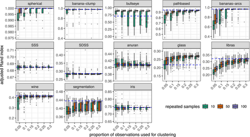
The proportion () of included in can impact the variability of the clustering performance. When is large, is necessarily small for computational practicality, and there is far more variability in the clustering. To alleviate the effects of this variation, we propose running the partitioning algorithm on several () different versions of , and choosing the result which minimizes (1) on the entire dataset after classifying , which can be done in parallel. We study these suggestions in Section 3.4.
3 Performance Evaluations
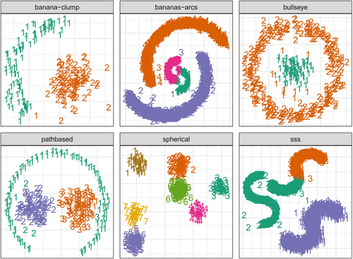
We evaluated our improvements to -means in terms of six synthetic 2D datasets from [37], shown in Figure 3, the subset of the Sloan Digital Sky Survey (SDSS) dataset in [38], and six real-world classification datasets from the UCI Machine Learning Repository [39], with details in Table 1.
| Adjusted Rand Index | ||||||
|---|---|---|---|---|---|---|
| Data set | Naive | AAC | OTQT | |||
| spherical | 7 | 500 | 2 | 1.000 | 1.000 | 1.000 |
| banana-clump | 2 | 200 | 2 | 0.980 | 0.980 | 0.980 |
| bullseye | 2 | 400 | 2 | 0.710 | 0.710 | 0.710 |
| pathbased | 3 | 300 | 2 | 0.939 | 0.939 | 0.939 |
| bananas-arcs | 4 | 4515 | 2 | 0.966 | 0.966 | 0.966 |
| SSS | 3 | 5015 | 2 | 0.685 | 0.685 | 0.685 |
| SDSS | 2 | 1507 | 5 | 0.286 | 0.286 | 0.286 |
| anuran | 10 | 7195 | 22 | 0.407 | 0.408 | 0.408 |
| glass | 7 | 214 | 9 | 0.268 | 0.206 | 0.217 |
| libras | 15 | 360 | 90 | 0.302 | 0.314 | 0.322 |
| wine | 3 | 178 | 13 | 0.416 | 0.416 | 0.416 |
| segmentation | 7 | 2310 | 19 | 0.436 | 0.437 | 0.436 |
| iris | 3 | 150 | 4 | 0.744 | 0.744 | 0.744 |
Our evaluations were on the naive and our AAC and OTQT approaches, with all methods efficiently coded in C with R [29] interfaces in our kkmeans package. Numerical clustering performance was assessed by the adjusted Rand Index (ARI) [40] that compared the grouping obtained by each algorithm with the true partition. The ARI takes values no greater than unity, with values closer to unity indicating good clustering performance.
3.1 Performance of AAC and OTQT Algorithms
3.1.1 Clustering Performance
The clustering performance of all three methods is summarized, numerically for all datasets in Table 1, and also visually for the 2D datasets in Figure 3. For each of the datasets from [37] and the SDSS data, all three methods arrived at the same final partition after initializations. The naive, AAC, and OTQT methods each performed the best on one UCI dataset each, and yielded the same result on two datasets. On the remaining dataset anuran, the AAC and OTQT methods yielded the same solution that is marginally better than that of the naive method.
3.1.2 Timing Results
Figure 4 displays the change in time taken by AAC and OTQT, relative to the naive method, to arrive at the terminating solution for the datasets in Table 1, with all three methods started from each of the initializations. Excepting the spherical and glass datasets, the naive method typically takes the longest time to termination. In general, the AAC and OTQT methods take similar amounts of time, with AAC narrowly faster in slightly more cases. Thus, the naive method is fastest for datasets with fewer average observations per cluster, while OTQT is at the other end of the spectrum. Because computational overhead in the algorithms increases from the naive to the AAC to the OTQT, our results suggest using algorithms in that order accordingly as the average number of observations increases. In essence, AAC or OTQT calculations make sense only when their use can be justified, which happens when is larger.

3.2 Comparison of Different Kernel Functions
Table 2 compares results obtained using the four kernels described in Section 2.1. We see that the Gaussian kernel generally performs well across the variety of datasets used in this evaluation. However, in some instances, the Laplace kernel is the best performer, and indeed, on the SDSS dataset, vastly outperforms the others. The polynomial and sigmoid kernels generally underperform relative to the other two kernels, but there are some datasets where the sigmoid kernel performs well: indeed, it is a runaway winner on the SSS dataset.
| Adjusted Rand Index | ||||
|---|---|---|---|---|
| Data set | Gaussian | Laplace | Polynomial | Sigmoid |
| spherical | 1.000 | 0.996 | 1.000 | 0.898 |
| banana-clump | 1.000 | 1.000 | 0.980 | 0.980 |
| bullseye | 0.619 | 0.080 | 0.013 | −0.002 |
| pathbased | 0.930 | 0.929 | 0.425 | 0.401 |
| bananas-arcs | 0.951 | 0.520 | 0.378 | 0.463 |
| SSS | 0.673 | 0.741 | 0.749 | 0.972 |
| SDSS | 0.893 | 0.985 | 0.051 | 0.353 |
| glass | 0.268 | 0.219 | 0.229 | 0.021 |
| libras | 0.315 | 0.274 | 0.289 | 0.272 |
| wine | 0.416 | 0.416 | 0.382 | 0.171 |
| segmentation | 0.436 | 0.502 | 0.413 | 0.346 |
| iris | 0.758 | 0.731 | 0.640 | 0.530 |
3.3 Computational Complexity Analysis
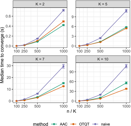
We next empirically evaluated the effect of and on the time taken for each algorithm to converge. We systematically generated datasets via R's MixSim [41] package. In all, 400 datasets were generated for each combination of and . These 400 datasets had dimensions evenly split with . Note that does not affect runtime, as the Gram matrix for each dataset is computed and stored before clustering, and therefore adds the same constant time for each method. All datasets were generated with a small amount of overlap among the clusters, with a generalized overlap value [42] equal to . Similar to the comparisons between algorithms in previous sections, within each of the datasets all three clustering algorithms began at the same initial values.
Figure 5 displays the median time to converge for each parameter combination. In general, the AAC and OTQT methods outperform the naive method, with the improvement becoming more pronounced for larger datasets. When there are only two clusters, we see that the added overhead present in the OTQT method means that it takes longer than the AAC method. Since there are only two clusters, the QT step is unnecessary, and thus it is recommended to use the AAC method in these situations. When the number of clusters increases, however, the time efficiency of the OTQT method is realized. In particular, as the number of clusters increases, the OTQT method continues to converge faster than the AAC method, as the QT step is designed to reduce the total number of comparisons required in each pass through the dataset.
3.4 Evaluating the SCAC Strategy for Larger Datasets
We evaluated SCAC on the datasets of Table 1, with -means clustering done using OTQT. We can perform -means clustering on the entire datasets here (as was done in Section 3.1) so here our investigation is determining how SCAC can perform relative to clustering of the entire sample. Section S2 illustrates performance on the bananas-arcs dataset. Figure S1 shows performance of the SCAC strategy on one realization with set at 5% of . We see that the first SCAC run happens to do quite well (ARI = 0.954) but the next five SCAC runs, with ARIs ranging from 0.606 to 0.964, indicate substantial variability in the clustering performance. We therefore evaluate performance of SCAC over different , and . Figure 6 displays the results on each of the datasets for different and . We see that as both and increase, the resulting ARI matches more closely that from the partitioning obtained using the complete dataset, with decreasing variance. This effect depends on the dimension of the dataset, as datasets with higher dimension require a larger proportion of the original dataset to achieve better results. For many low-dimensional datasets we see that even the smallest size of yields similar results to clustering the entire dataset, especially with a large number of repeated samples. While the choice of will likely be dictated by availability of compute resources, we recommend using larger for smaller to achieve better results. We apply SCAC in the next section.
4 Color Quantization of Images
Color quantization is used to represent digital images by means of a few colors without appreciably degrading their visual quality [19]. It is useful for storing and transmitting data. Traditionally, color quantization has been done in the RGB colorspace, where -means has been a method of choice, but some authors [43] have used it in human perception-based colorspaces. Indeed, [44] showed in an expansive study that -means color quantization is better done in these colorspaces in many cases. However, they also expressed some misgivings on the use of -means in these colorspaces given that these spaces have features that are very different from each other. We therefore investigate the use of -means on color quantization of five different publicly available images.
We performed color quantization using both our -means and -means algorithms on RGB, HCL, and CIEXYZ colorspace, with colors, and with each variable being scaled prior to clustering. For -means, the entire set of colors was used, while for -means, we used our SCAC strategy with and .
Figure 7 illustrates performance on Statlab. We display only the results with colors in the CIEXYZ space, which is the space where it performs best using both -means and -means. While both algorithms perform fairly similarly, the 64 colors chosen to describe the image differ and emphasize different features of each image. In particular, the -means quantized images have fewer colors in the background of the signpost, creating a less pixelated look and a clearer distinction with the text compared to the results from -means. Beyond visual displays, we also assessed the quality of the quantized image in faithfully representing the original image in terms of the Visual Information Fidelity (VIF) criterion [45] that takes values in (0,1) with 1 representing perfect fidelity and values farther away from unity representing increased degradation. VIF compares two images using natural scene statistics and shows the perceptual quality difference between them, and in particular, is better suited for images with natural scenes. The VIF for the -means quantized image is slightly higher than that obtained using -means image.

We also explored the use of -means in the different colorspaces in a few more images of different sizes, displayed in Figure 8, with results on the VIF obtained using the two methods in the three colorspaces for displayed in Figure 9 and Table S3. For smaller palettes (), there is not much benefit to leaving the RGB colorspace, but for larger numbers of colors, CIEXYZ seems to be better for quantization. In all cases, HCL is the worst performer. Between -means and -means, the honors are shared, so we now try and see whether we can explain performance in terms of the characteristics of the images.

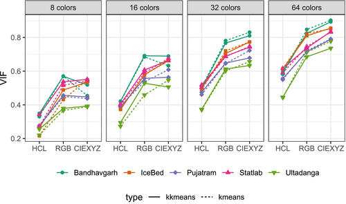
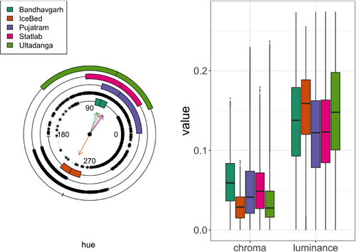
Figure 10 displays circular-linear boxplots of the distributions of unique colors for our images in terms of hue (H), chroma (C) and luminance (L). Hue being an angular quantity, we use circular boxplots [46, 47] to display its distribution, while linear boxplots are used for the C and L bands. In general, we see that Bandhavgarh is the worst performer for -means. The C-distribution here is highly skewed in the clockwise direction, with high kurtosis but low IQR. The other two values are fairly symmetric, however. The best performer, IceBed, has a relatively symmetric distribution for H and C, with L only slightly skewed toward smaller values. Pujatram and Statlab both perform best for two of the four colors, but overall have relatively equal performance between the methods and indeed, their distributions are only slightly skewed (but in opposite directions). They have similar-looking distributions for the hue, with both of them being skewed toward higher values. Lastly, Ultadanga is best suited for -means in the three higher colors (), has a symmetric distribution for H and L, and is only slightly skewed in C. In summary, it seems that -means performs best when the distributions for each of H, C, and L are symmetric, and poorly with increased circular skewness in H, but is more robust to skewness in the L band. Our initial findings here call for a deeper analysis that is beyond the scope of this paper.
5 Conclusions
This paper delivers computational improvements to the -means algorithm using AAC and OTQT approaches. As with -means [32] and -modes [12] algorithms, we provide theoretical guarantees for the OT version, while the OTQT algorithm's generally good performance is demonstrated through experiments on 2D synthetic and higher-dimensional real-world classification datasets. We also use our approach to study the performance of -means in the color quantization of images in human perception-based colorspaces. A R package implements the naive, AAC and OTQT methods as well as methods for estimating the bandwidth parameter for the Gaussian kernel using both MKNN and MATR.
There are a number of issues that can benefit from further study. For instance, the problem of selecting an optimal number of clusters using -means remains unresolved. Also unresolved are penalization methods for in (1) based on the complexity of the transformation, where the challenge is accentuated by the fact that the Jacobian is unclear since is a potentially infinite-dimensional function of complicated form. Thus we see that while we have made important computational improvements to -means algorithms, there remain questions worthy of further attention.
Author Contributions
Joshua D. Berlinski wrote the R package, developed the methodology, proved the claim and performed the computations. Ranjan Maitra conceptualized the problem and planned the framework and the experiments, and the applications. Both authors shared in the writing of the article.
Acknowledgments
We thank the Editor-in-Chief for comments on an earlier version that improved this article. All original digital images were converted to the Tagged Image File Format (TIFF). Statlab is a 2023 digital photograph of a plaque that stands outside the building housing Iowa State University's Department of Statistics. The plaque commemorates the 1933 establishment there of the first statistical laboratory in the United States of America. IceBed is thanks to Nima Sarikhani's dreamy photograph, named “Ice Bed”, of a young polar bear drifting to sleep on a bed carved into an iceberg, first published on February 7, 2024. Bandhavgarh is courtesy of Staffan Widstrand of the World Wildlife Foundation and shows a Royal Bengal tiger in Bandhavgarh National Park, India. Pujatram is a photograph, released by the transport department of the Government of West Bengal, India, of a specially decorated 2023 tram commemorating both the 150th anniversary of Calcutta Tramways and the then-recent award of UNESCO's intangible cultural heritage tag to Kolkata's (formerly, Calcutta) famed Durga Puja festival. Ultadanga is a photograph in December 2010 of the multimodal traffic chaos at the Ultadanga-VIP Road intersection in Kolkata, India. Statlab and Ultadanga are from the second author's personal photographs collection. The research of the second author was supported in part by the United States Department of Agriculture (USDA) National Institute of Food and Agriculture (NIFA) Hatch project IOW03717. The content of this paper is however solely the responsibility of the authors and does not represent the official views of the USDA. Open access funding provided by the Iowa State University Library.
Conflicts of Interest
The authors declare no conflicts of interest.
Open Research
Data Availability Statement
The data that supports the findings of this study are both publicly available and also from the Supporting Information materials section of this article.


