International Journal of Robust and Nonlinear Control

Volume 33, Issue 12 pp. 6734-6753

RESEARCH ARTICLE

Open Access

Design of input assignment and feedback gain for re-stabilizing undirected networks with High-Dimension Low-Sample-Size data

Hitoshi Yasukata,

Hitoshi Yasukata

orcid.org/0009-0004-6816-4471

Department of Systems and Control Engineering, School of Engineering, Tokyo Institute of Technology, Tokyo, Japan

Search for more papers by this author

Xun Shen,

Xun Shen

orcid.org/0000-0002-8827-5791

Department of Systems and Control Engineering, School of Engineering, Tokyo Institute of Technology, Tokyo, Japan

Search for more papers by this author

Hampei Sasahara,

Corresponding Author

Hampei Sasahara

[email protected]

Department of Systems and Control Engineering, School of Engineering, Tokyo Institute of Technology, Tokyo, Japan

Correspondence Hampei Sasahara, Department of Systems and Control Engineering, School of Engineering, Tokyo Institute of Technology, 2-12-1 Ookayama, Tokyo, 152-8522, Japan.

Email: [email protected]

Search for more papers by this author

Jun-ichi Imura,

Jun-ichi Imura

Department of Systems and Control Engineering, School of Engineering, Tokyo Institute of Technology, Tokyo, Japan

Search for more papers by this author

Makito Oku,

Makito Oku

Institute of Natural Medicine, University of Toyama, Toyama, Japan

Search for more papers by this author

Kazuyuki Aihara,

Kazuyuki Aihara

International Research Center for Neurointelligence (WPI-IRCN), The University of Tokyo, Tokyo, Japan

Search for more papers by this author

Hitoshi Yasukata,

Hitoshi Yasukata

orcid.org/0009-0004-6816-4471

Department of Systems and Control Engineering, School of Engineering, Tokyo Institute of Technology, Tokyo, Japan

Search for more papers by this author

Xun Shen,

Xun Shen

orcid.org/0000-0002-8827-5791

Department of Systems and Control Engineering, School of Engineering, Tokyo Institute of Technology, Tokyo, Japan

Search for more papers by this author

Hampei Sasahara,

Corresponding Author

Hampei Sasahara

[email protected]

Department of Systems and Control Engineering, School of Engineering, Tokyo Institute of Technology, Tokyo, Japan

Correspondence Hampei Sasahara, Department of Systems and Control Engineering, School of Engineering, Tokyo Institute of Technology, 2-12-1 Ookayama, Tokyo, 152-8522, Japan.

Email: [email protected]

Search for more papers by this author

Jun-ichi Imura,

Jun-ichi Imura

Department of Systems and Control Engineering, School of Engineering, Tokyo Institute of Technology, Tokyo, Japan

Search for more papers by this author

Makito Oku,

Makito Oku

Institute of Natural Medicine, University of Toyama, Toyama, Japan

Search for more papers by this author

Kazuyuki Aihara,

Kazuyuki Aihara

International Research Center for Neurointelligence (WPI-IRCN), The University of Tokyo, Tokyo, Japan

Search for more papers by this author

First published: 25 April 2023

https://doi.org/10.1002/rnc.6720

Share a link

Email
Wechat
Bluesky

Abstract

There exists a critical transition before dramatic deterioration of a complex dynamical system. Recently, a method to predict such shifts based on High-Dimension Low-Sample-Size (HDLSS) data has been developed. Thus based on the prediction, it is important to make the system more stable by feedback control just before such critical transitions, which we call re-stabilization. However, the re-stabilization cannot be achieved by traditional stabilization methods such as pole placement method because the available HDLSS data is not enough to get a mathematical system model by system identification. In this article, a model-free pole placement method for re-stabilization is proposed to design the optimal input assignment and feedback gain for undirected network systems only with HDLSS data. The proposed method is validated by numerical simulations.

1 INTRODUCTION

There always exist abrupt critical transitions before system deterioration in various complex network systems such as ecological systems, climate systems, power systems, and biological systems.¹ In these days, critical transition detection methods have been increasingly studied.^2-5 Chen et al.⁵ have proposed a method, called Dynamical Network Biomarker (DNB) theory, for predicting a critical transition from a healthy stage to a disease stage of a dynamical network in a living organism only with very few samples, referred to as High-Dimension Low-Sample-Size (HDLSS) data. In DNB theory, the progression of a disease is modeled as a system parameter shift of nonlinear dynamical systems and the critical transition is regarded as a bifurcation, but any information of the system model is not required. In a situation where a bifurcation is about to occur in the biological network system, the system state assigned to the nodes that constitute the subnetwork, called DNB nodes, show large fluctuations. The fluctuations of the DNB nodes can be captured only with HDLSS data, and we can detect the stage just before the bifurcation occurs. DNB theory is applied to various fields other than system biology to predict deterioration of a network system, which is called Dynamical Network Marker (DNM) theory in general sense.^6-9

The realization of critical transition detection stimulates research on methods to avoid the critical transition at the stage of the detection. Given the control theoretical approach, preventing a network system in a pre-deteriorating stage, which is the stage just before the critical transition occurs, from falling into a deteriorating stage is regarded as designing a controller that improves the stability degree by pole placement, which we call re-stabilization. If the mathematical model of the system is available, or can be identified from the measured data, then conventional control methods can be employed to enhance the stability degree of the system. However, it is difficult of obtain the entire system model for a large-scale complex network system. Moreover the available data is sometimes HDLSS, which is not enough to identify the dynamics.^{10, 11} For example, in the case of gene network systems, the dimension of microarray data of gene expression is almost tens of thousands while the sample size is a dozen or more at most.¹²

A few studies on re-stabilization can be found. A data-driven method to find the input assignment with maximal controllability Gramian has been proposed,¹³ which relates to minimal energy control. However, the method needs abundant data whose sample size is equal to the dimension of the state variable. Thus, the method cannot be applied to the case of HDLSS data. In a very recent study, approximate pole placement for gene network systems with HDLSS data has been proposed,¹⁴ based on Brauer's theorem.¹⁵ Although the method is suitable for HDLSS data, no theoretical analysis has been presented for exact characterization of the solution of the pole placement problem. Also, a single-input assignment design for undirected network systems with HDLSS data has been proposed,¹⁶ where the proposed input assignment is the optimal solution for minimizing the input energy. The research has also given the approximated control method. However, no theoretical discussion for the approximation has been developed.

In this article, for undirected network systems, we propose a method to design the optimal feedback gain and the optimal input assignment for feedback control that makes the system more stable under pre-deteriorating stage, called re-stabilization, without the system model which adopts two different criteria: minimizing input energy and minimizing the Frobenius norm of the feedback gain to be designed. Minimizing the input energy is one of the typical criterion for control problem since the control energy corresponds to the effort needed to control a network system.¹⁷ Minimizing the Frobenius norm of the feedback gain is also significant in the case of multi-input control, because small gains are beneficial to reduce energy consumption and noise amplification or improve the transient response, where the Frobenius norm is often used as a measure of the size of the gain.^18-20 For each case, we show that the optimal feedback gain and the optimal input assignment which shift the dominant eigenvalue of the Jacobian matrix away from the imaginary axis can be designed by only using the information derived from the HDLSS data of the state if the system is under the pre-deteriorating stage. Furthermore, we prove that the solution for minimizing input energy and the solution for minimizing the Frobenius norm of the feedback gain are equivalent, that is, the two problems can be solved in a unified manner. We also propose a practical design method in which the optimal feedback gain is approximated to be sparse with an analytic evaluation of the error caused by the approximation. In addition, we provide the specific algorithm for designing the input assignment and feedback gain by using HDLSS time-series data of the system.

The rest of the article is organized as follows. In Section 2, we give system description, a brief review of pre-deteriorating stage detection with HDLSS data, and the design criterion with the formal assumption. Section 3 presents the proposed method for minimizing input energy and for minimizing the Frobenius norm of feedback gain, the evaluation of the error of the practical design method, and the algorithm for the design. In Section 4, we show the proposed method is effective by numerical simulations. Finally, we conclude the article in Section 5.

2 PROBLEM DESCRIPTION

2.1 System description

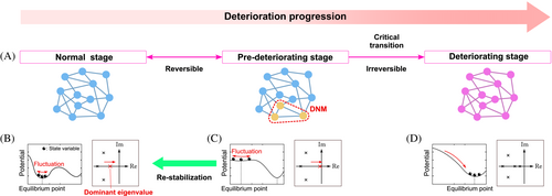
Figure 1A shows the progression of the deterioration of a complex network system. For example, it is known that deterioration of the gene regulatory networks may cause the organisms to fall into a disease stage.⁵ The progression can be divided into three stages: a normal stage, a pre-deteriorating stage, and a deteriorating stage. The deterioration of the network system of interest is not smooth but abrupt, that is, there exists a tipping point where the sudden shift from a normal stage to a deteriorating stage occurs. We define a pre-deteriorating stage as the limit of a normal stage immediately before the tipping point is reached. The process from a normal stage to a pre-deteriorating stage is reversible while the process from a pre-deteriorating stage to a deteriorating stage is irreversible or very difficult. Mathematically, a deterioration progression of a system is regarded as a slow change of a bifurcation parameter of a system.⁵ The dynamical evolution of the system for some value of a bifurcation parameter

\mu

is expressed as follows:

\dot{z}(t)=f\left(z(t);\mu \right)+\omega (t),

(1)

where

z(t)\in {\mathbb{R}}^n

denotes the state of the system,

f:{\mathbb{R}}^n\to {\mathbb{R}}^n

is a nonlinear function, and

\omega (t)\in {\mathbb{R}}^n

is a white Gaussian noise with zero means and covariance matrix

D\in {\mathbb{R}}^{n\times n}

. Let

{z}_e\left(\mu \right)

be an equilibrium state with respect to the noiseless autonomous system

\dot{z}=f\left(z;\mu \right)

, and assume that

f

can be linearly approximated in the neighborhood of

z={z}_e\left(\mu \right)

. Then, the linear approximation of the system around

{z}_e\left(\mu \right)

is written as

\dot{x}(t)= Ax(t)+\omega (t),

(2)

where

x(t)=z(t)-{z}_e\left(\mu \right)

A\in {\mathbb{R}}^{n\times n}

is the Jacobian matrix

{\left.\frac{\partial f\left(z,u\right)}{\partial z}\right|}_{z={z}_e\left(\mu \right)}

, which depends on the value of

\mu

. The eigenvalue of

A

with the largest real part, called the dominant eigenvalue, determines the stability degree of the system. Let

{\mathcal{M}}_{\mathrm{n}}

be an open set of the bifurcation parameter

\mu

such that the system is under a normal stage. When

\mu ={\mu}_{\mathrm{n}}\in {\mathcal{M}}_{\mathrm{n}}

, the system is under a normal stage and the real part of the dominant eigenvalue of

A

is negative and relatively further from zero. Thus, the equilibrium point

{z}_e\left({\mu}_{\mathrm{n}}\right)

is stable and the fluctuation of the state caused by external noises is relatively small (see Figure 1B). Let

\partial {\mathcal{M}}_{\mathrm{n}}

be the boundary of

{\mathcal{M}}_{\mathrm{n}}

and

{\mu}_{\mathrm{pre}}

denotes a bifurcation parameter such that

{\mu}_{\mathrm{pre}}\in {\mathcal{M}}_{\mathrm{n}}

and

{\mu}_{\mathrm{pre}}\approx {\mu}_{\mathrm{crit}}\in \partial {\mathcal{M}}_{\mathrm{n}}

. When

\mu

reaches

{\mu}_{\mathrm{pre}}

, the system is under a pre-deteriorating stage and the real part of the dominant eigenvalue of

A

is very close to zero. Thus,

{z}_e\left({\mu}_{\mathrm{pre}}\right)

is still stable but the system is sensitive to external noises, that is, the fluctuation becomes large (see Figure 1C). Although the equilibrium point

{z}_e\left(\mu \right)

changes as the change of the bifurcation parameter

\mu

, the change of

{z}_e\left(\mu \right)

is regarded as continuous and relatively small when

\mu \in {\mathcal{M}}_{\mathrm{n}}

. On the other hand, when

\mu

reaches

{\mu}_{\mathrm{crit}}\in \partial {\mathcal{M}}_{\mathrm{n}}

and gets out of

\partial {\mathcal{M}}_{\mathrm{n}}\cup {\mathcal{M}}_{\mathrm{n}}

, a critical transition occurs and the state can change abruptly to another equilibrium point. Then, the system becomes under a deteriorating stage, where the equilibrium point is far from

{z}_e\left({\mu}_{\mathrm{n}}\right)

and

{z}_e\left({\mu}_{\mathrm{pre}}\right)

(see Figure 1D).

Details are in the caption following the image — **FIGURE 1**
Open in figure viewer PowerPoint

Schematic illustration of the dynamical features of deterioration progression. (A) The progression from a normal stage to a deteriorating stage. (B) The potential function and the poles of the system under a normal stage. A normal stage is a steady state, where the system is robust and resilient. (C) The potential function and the poles of the system under a pre-deteriorating stage. A pre-deteriorating stage is situated just before the bifurcation, where the system shows large fluctuations due to noises. (D) The potential function and the poles of the system under a deteriorating stage. A deteriorating stage is a stable state, where the system is robust and resilient, similarly to a normal stage.

2.2 Pre-deteriorating stage detection with HDLSS data

A pre-deteriorating stage detection method has been proposed.^{5, 8, 9} Based on the theoretical analysis presented by Chen et al.,⁵ the system under a pre-deteriorating stage shows some generic properties: there exists a group of nodes whose standard deviation drastically increases, and the covariance between every pair within the group also increases drastically in absolute value. This group represents the dynamical features of the network system and the nodes in the group are expected to form a subnetwork. Then, this subnetwork is regarded as a DNM and a node in the subnetwork is called a DNM node. The existence of DNM nodes implies that the system is under the pre-deteriorating stage.

We provide the details of the theoretical analysis of the system properties under a pre-deteriorating stage, which is based on Lyapunov equation. If a network system is under a pre-deteriorating stage, the following assumption holds:

Assumption 1.The system matrix $A\in {\mathbb{R}}^{n\times n}$ is stable and the dominant eigenvalue ${\lambda}_1\in \mathbb{C}$ satisfies $\operatorname{Re}\left({\lambda}_1\right)\approx 0$ .

Here, $\mathbb{C}$ denotes the set of complex numbers. In addition, this article focuses on undirected networks, that is, the system matrix $A$ is symmetric and all the eigenvalues are real, which is described by the following technical assumption:

Assumption 2.The system matrix $A$ is symmetric and diagonalizable, and the eigenvalues ${\lambda}_i\kern0.3em \left(i=1,\dots, n\right)$ satisfy ${\lambda}_n<{\lambda}_{n-1}<\cdots <{\lambda}_2<{\lambda}_1$ .

Since

A\in {\mathbb{R}}^{n\times n}

is symmetric and diagonalizable, there exists an orthogonal matrix

V\in {\mathbb{R}}^{n\times n}

that satisfies

A=V\Lambda {V}^T

, where

\Lambda =\operatorname{diag}\left\{{\lambda}_1,{\lambda}_2,\dots, {\lambda}_n\right\}

and the column vectors are normalized. Note that the column vectors of

V

are the eigenvectors of

A

. Let

C\in {\mathbb{R}}^{n\times n}

be the covariance matrix of

x

at steady state. Then, for the element of

C

, if

V\left(i,1\right)\ne 0

and

V\left(j,1\right)\ne 0

, the following holds:²¹

\underset{\lambda_1\to -0}{\lim}\mid C\left(i,j\right)\mid =\infty,

(3)

where

{\lambda}_1\to -0

denotes the one-sided limit of

{\lambda}_1

from below. Equation (3) implies the generic properties of a gene network system. If

V\left(i,1\right)\ne 0

, the standard deviation of node

i

is extremely large at the pre-deteriorating stage. Furthermore, if

V\left(i,1\right)\ne 0

and

V\left(j,1\right)\ne 0

, the covariance of node

i

and node

j

is extremely large in absolute value under the pre-deteriorating stage.

From the above discussion, node $i$ such that $V\left(i,1\right)\ne 0$ shows large fluctuation under the pre-deteriorating stage. Note that $V\left(i,1\right)$ is the $i$ th element of the eigenvector of $A$ corresponding to the dominant eigenvalue ${\lambda}_1$ . Here, we define the dominant eigenvector as follows:

Definition 1.The vector ${v}_1$ is called the dominant eigenvector of $A$ if $A{v}_1={\lambda}_1{v}_1$ for the dominant eigenvalue ${\lambda}_1$ of $A$ .

Then, the nodes corresponding to the non-zero element of the dominant eigenvector are with large fluctuations under the pre-deteriorating stage. We can capture the large fluctuation and identify the dominant eigenvector only with HDLSS data following the procedure explained in Section 3.1.

2.3 Design criterion

After detecting a pre-deteriorating stage, the next goal is to prevent the system from shifting to a deteriorating stage and bring it back to the normal stage, which we refer to as re-stabilization in this article. When the system is under a pre-deteriorating stage, the real part of the dominant eigenvalue of the system matrix, which corresponds to the linearization around ${z}_e\left({\mu}_{\mathrm{pre}}\right)$ , is close to zero. If the dominant eigenvalue of the system matrix is shifted away from zero, the system matrix becomes more stable. Then, the original nonlinear system also becomes more stable where the equilibrium point is still close to ${z}_e\left({\mu}_{\mathrm{pre}}\right)$ , that is, the re-stabilization can be achieved. Therefore, we consider the problem to shift the dominant eigenvalue away from zero based on pole placement method.

We formulate the re-stabilization problem assuming that some parameters of the system matrix can be adjusted. For example, in gene regulatory networks, gene knockdown, and gene overexpression can be implemented to adjust the system parameters.²² Naturally, two questions arise: which nodes should be targeted? How much the corresponding parameters should be adjusted? By regarding the perturbation matrix as a multiplication of the system input matrix and a feedback gain matrix, we address the questions as a problem of designing these two matrices.

The system (2) with an input term is written as follows:

\dot{x}(t)= Ax(t)+ Bu(t)+\omega (t),

(4)

where

u\in {\mathbb{R}}^m

is an input vector and

B\in {\mathbb{R}}^{n\times m}

is an input assignment, which can be designed arbitrarily. For the system matrix

A

which satisfies Assumptions 1 and 2, we set the requirements for a pole placement as follows:

The dominant eigenvalue ${\lambda}_1$ is shifted to ${\lambda}_1-{\lambda}_{\mathrm{shift}}$ ;
The eigenvalues ${\lambda}_2,{\lambda}_3,\dots, {\lambda}_n$ and the corresponding eigenvectors do not change,

where

{\lambda}_{\mathrm{shift}}

is a positive real number and satisfies

{\lambda}_1-{\lambda}_{\mathrm{shift}}>{\lambda}_2

. Then, let

𝒦 (B, λ_{shift})

be the set of feedback gains

K\in {\mathbb{R}}^{m\times n}

that realize a pole placement that satisfies the above requirements for a given input assignment

B

and

{\lambda}_{\mathrm{shift}}

. The state feedback with respect to

K \in 𝒦 (B, λ_{shift})

is written as follows:

u= Kx.

(5)

We define two cost functions and determine the optimal input assignment and the optimal feedback gain with respect to each function. One is the input energy

{J}_1:= {\int}_0^{\infty }{u}^Tu\kern0.3em dt,

(6)

with

\omega (t)=0

, and the other one is the Frobenius norm of feedback gain

{J}_2:= {\left\Vert K\right\Vert}_F.

(7)

Here,

{J}_1

depends on the initial value of

x(t)

. Minimizing the Frobenius norm of feedback gain corresponds to minimizing the amount of change of the value of components of the system matrix, which is supposed to reduce the load of the system caused by the input. Let

{B}^{\ast }

and

{K}^{\ast }

be the optimal

B

and

K

, which minimize

{J}_1

for all the initial state

x(0)

, or

{J}_2

. Note that

{K}^{\ast }

depends on

{B}^{\ast }

since feedback gains that realize the above pole placement depend on

B

The available data for the design of $B$ and $K$ is the time-series data of all the nodes at the steady state with sample size $N$ , which is expressed as ${\tilde{Z}}_N=\left\{z\left({t}_0\right),\dots, z\left({t}_{N-1}\right)\right\}$ . For some systems, such as power systems or biological systems, the sample size $N$ is much smaller than the dimension $n$ of $z(t)$ .^10-12 Data with such property is called HDLSS data, defined as follows:

Definition 2.Data ${\tilde{Z}}_N=\left\{z\left({t}_0\right),\dots, z\left({t}_{N-1}\right)\right\}$ is called HDLSS data if the sample size $N$ and the dimension $n$ of $z(t)$ satisfy $N\ll n$ .

Since the measured data with a sample size greater than or equal to the dimension of $z(t)$ are required for system identification, we cannot identify the system matrix $A$ by using HDLSS data. On the other hand, we can obtain the HDLSS data of the state $x(t)=z(t)-{z}_e$ since we can estimate the equilibrium point ${z}_e$ from the steady state data of $z(t)$ .

Summarizing the above discussion, the problem we address here is to design the appropriate input assignment $B$ and the appropriate feedback gain $K$ with respect to minimizing ${J}_1$ or ${J}_2$ under Assumptions 1 and 2.

3 PROPOSED METHOD

In this section, we present a method for designing the appropriate input assignment and the appropriate feedback gain, which can be achieved only with the HDLSS data of $x$ .

3.1 Available information

According to the existing results,^{21, 23} we can obtain some of the essential information about the system matrix

A

from HDLSS data of

x(t)

. Let

C\in {\mathbb{R}}^{n\times n}

be the covariance matrix of

x

at steady state. Then, under Assumption 1, the following holds:²¹

\underset{\lambda_1\to 0}{\lim}\left(-2{\lambda}_1\right)C\propto {v}_1{v}_1^T.

(8)

This relation implies that the dominant eigenvector of

C

converges to the dominant eigenvector

{v}_1

A

{\lambda}_1

approaches to zero. Since

{\lambda}_1\to 0

corresponds to

\mu \to {\mu}_{\mathrm{crit}}

, if the system is at a pre-deteriorating stage, that is,

\mu ={\mu}_{\mathrm{pre}}

, the dominant eigenvector of

C

is approximately equal to

{v}_1

A

with

\mu ={\mu}_{\mathrm{pre}}

. In addition, the formula (8) also implies that

{\eta}_1\to \infty

and

\operatorname{rank}(C)\to 1

{\lambda}_1\to 0

, where

{\eta}_1

denotes the dominant eigenvalue of

C

. Although the covariance matrix

C

x

is not available with HDLSS data of

x

, we can estimate the dominant eigenvector of

C

under certain conditions: if

{\eta}_1

is sufficiently large and outstanding compared to the other eigenvalues of the covariance matrix

C

, the dominant eigenvector of the sample covariance matrix

\tilde{C}

of HDLSS data of

x

can be treated as an approximated vector of the dominant eigenvector of

C

.²³ Therefore, we can obtain an approximated vector of the dominant eigenvector

{v}_1

A

with HDLSS data of

x

under a pre-deteriorating stage.

3.2 Problem formulation

From the above discussion, under Assumptions 1 and 2, we assume that ${v}_1$ is available. Therefore, for minimizing ${J}_1$ , the problem we address is formulated as follows:

Problem 1.For the system (4), suppose Assumptions 1 and 2 hold and the dominant eigenvector ${v}_1$ of $A$ is available. Then, derive the optimal solution $\left({B}^{\ast },{K}^{\ast}\right)$ of the following optimization problem (P₁) by using ${v}_1$ :

|\begin{array}{l} variables & B, K \\ minimize & J_{1} for all x (0) \in ℝ^{n} \\ subject to & B \in ℬ, \\ K \in 𝒦 (B, λ_{shift}), \end{array}

(P₁)

where

\mathcal{B}

is some feasible set of

B

Similarly, we call Problem 2 for the problem where “ ${J}_1$ for all $x(0)\in {\mathbb{R}}^n$ ” is replaced by “ ${J}_2$ ” in Problem 1.

3.3 Optimal design with the dominant eigenvector of the system matrix

For an arbitrary feasible set $\mathcal{B}$ , Problems 1 and 2 can be solved by using the following theorem:

Theorem 1.For the system (4), suppose Assumptions 1 and 2 hold. Then, the optimization problem (P₁) is equivalent to the optimization problem in Problem 2, and that solution $\left({B}^{\ast },{K}^{\ast}\right)$ is given as follows:

{B}^{\ast }=\underset{B\in \mathcal{B}}{\arg\;\max}\left\Vert {v}_1^TB\right\Vert, \kern0.5em

(9)

{K}^{\ast }=-\frac{\lambda_{\mathrm{shift}}}{{\left\Vert {v}_1^T{B}^{\ast}\right\Vert}^2}{B^{\ast}}^T{v}_1{v}_1^T,\kern0.5em

(10)

where

\mathcal{B}

is an arbitrary feasible set of

B

and

{v}_1

is the dominant eigenvector of the system matrix

A

Proof of Theorem 1.Because $A$ is a real symmetric matrix, there exists an orthogonal matrix $V$ such that

A=V\Lambda {V}^T,\kern0.5em

(11)

\Lambda =\operatorname{diag}\left\{{\lambda}_1,{\lambda}_2,\dots, {\lambda}_n\right\},\kern0.5em

(12)

and its column vectors are normalized. Now, let

\hat{A}

be the system matrix of the closed-loop system with the state feedback (5). Then, the following equation holds:

\begin{array}{ll}\hat{A}& =A+ BK\\ {}& =V\Lambda {V}^T+ BK.\end{array}

(13)

The condition that the dominant eigenvalue

{\lambda}_1

is shifted to

{\lambda}_1-{\lambda}_{\mathrm{shift}}

and the other eigenvalues and its corresponding eigenvectors are not changed is equivalent to the condition that there exists a vector

\hat{v}

such that

\hat{A}\hat{v}\kern0.5em =\left({\lambda}_1-{\lambda}_{\mathrm{shift}}\right)\hat{v},

(14)

\hat{A}{v}_i\kern0.5em ={\lambda}_i{v}_i\kern1em \left(i=2,\dots, n\right),

(15)

where

{v}_i\kern0.3em \left(i=2,\dots, n\right)

is the

i

th column vector of

V

. Note that

\hat{v}

is determined by

\left({B}^{\ast },{K}^{\ast}\right)

but still has the arbitrary of constant multiple. By using (13), these equations are written in one equation as follows:

BK\left[\hat{v}\kern0.5em {v}_2\kern0.5em \cdots \kern0.5em {v}_n\right]=\left[\begin{array}{cccc}-V\left(\Lambda -\left({\lambda}_1-{\lambda}_{\mathrm{shift}}\right)I\right){V}^T\hat{v}& O& \cdots & O\end{array}\right].

(16)

On the other hand, because the eigenvalues of $\hat{A}$ are all real and distinct, there exists a non-singular matrix $\hat{V}$ such that

\hat{V}\kern0.5em =\left[\begin{array}{cccc}\hat{v}& {v}_2& \cdots & {v}_n\end{array}\right],

(17)

\hat{A}\kern0.5em =\hat{V}\hat{\Lambda}{\hat{V}}^{-1},

(18)

\hat{\Lambda}=\operatorname{diag}\left\{{\lambda}_1-{\lambda}_{\mathrm{shift}},{\lambda}_2,\dots, {\lambda}_n\right\}.\kern0.5em

(19)

Now, let

{\hat{w}}_1^T

be the first row vector of

{\hat{V}}^{-1}

. Then, from

{\hat{V}}^{-1}\hat{V}=I

, the following equation holds:

{\hat{w}}_1^T\hat{V}=\left[{\hat{w}}_1^T\hat{v}\kern0.5em {\hat{w}}_1^T{v}_2\kern0.5em \cdots \kern0.5em {\hat{w}}_1^T{v}_n\right]=\left[\begin{array}{cccc}1& 0& \cdots & 0\end{array}\right].

(20)

Therefore, we obtain

{\hat{w}}_1^T\hat{v}\kern0.5em =1,

(21)

{\hat{w}}_1^T{v}_i\kern0.5em =0\kern1em \left(i=2,\dots, n\right).

(22)

(22) implies that

{\hat{w}}_1

is orthogonal to

{v}_i\kern0.3em \left(i=2,\dots, n\right)

. Since

{v}_1,\dots, {v}_n

are orthogonal to each other, the following holds:

{\hat{w}}_1\in \mathrm{Span}\left\{{v}_1\right\}.

(23)

Furthermore, because of the arbitrary of constant multiple of

\hat{v}

, there exists the vector

\hat{v}

such that

{v}_1^T\hat{v}=1.

(24)

In this case, by using (21) and (23), the following holds:

{\hat{w}}_1={v}_1.

(25)

Then, by using (16), (17), and (25), we have

\begin{array}{ll} BK& =\left[-V\left(\Lambda -\left({\lambda}_1-{\lambda}_{\mathrm{shift}}\right)I\right){V}^T\hat{v}\kern0.5em O\kern0.5em \cdots \kern0.5em O\right]{\hat{V}}^{-1}\\ {}& =-V\left(\Lambda -\left({\lambda}_1-{\lambda}_{\mathrm{shift}}\right)I\right){V}^T\hat{v}{v}_1^T.\end{array}

(26)

From the above, the following formula holds:

K \in 𝒦 (B, λ_{shift}) \Rightarrow \exists \hat{v}; B K = - V (Λ - (λ_{1} - λ_{shift}) I) V^{T} \hat{v} v_{1}^{T}, v_{1}^{T} \hat{v} = 1 .

(27)

Moreover, by substituting (26) to (13) and using (24), we obtain (14) and (15). Thus, the following holds:

K \in 𝒦 (B, λ_{shift}) \Leftrightarrow \exists \hat{v}; B K = - V (Λ - (λ_{1} - λ_{shift}) I) V^{T} \hat{v} v_{1}^{T}, v_{1}^{T} \hat{v} = 1 .

(28)

Then, the optimization problem (P₁) is rewritten as follows:

\left|\kern1em \begin{array}{cccc}& \mathrm{variables}& & B,K\\ {}& \operatorname{minimize}& & {J}_1\kern0.3em \mathrm{for}\kern0.3em \mathrm{all}\kern0.3em x(0)\in {\mathbb{R}}^n\\ {}& \mathrm{subject}\kern0.3em \mathrm{to}& & B\in \mathcal{B}, \\ {}& & & \exists \hat{v};\kern0.3em BK=-V\left(\Lambda -\left({\lambda}_1-{\lambda}_{\mathrm{shift}}\right)I\right){V}^T\hat{v}{v}_1^T,\kern0.3em {v}_1^T\hat{v}=1.\end{array}\right.

(P₂)

Similarly, the optimization problem for minimizing

{J}_2

is written as follows:

\left|\kern1em \begin{array}{cccc}& \mathrm{variables}& & B,K\\ {}& \operatorname{minimize}& & {J}_2\\ {}& \mathrm{subject}\kern0.3em \mathrm{to}& & B\in \mathcal{B}, \\ {}& & & \exists \hat{v};\kern0.3em BK=-V\left(\Lambda -\left({\lambda}_1-{\lambda}_{\mathrm{shift}}\right)I\right){V}^T\hat{v}{v}_1^T,\kern0.3em {v}_1^T\hat{v}=1.\end{array}\right.

(P₃)

Now, for the optimization problem (P₂), we fix the input assignment $B$ and consider the following subproblem:

\left|\kern1em \begin{array}{cccc}& \mathrm{variables}& & K\\ {}& \operatorname{minimize}& & {J}_1\kern0.3em \mathrm{for}\kern0.3em \mathrm{all}\kern0.3em x(0)\in {\mathbb{R}}^n\\ {}& \mathrm{subject}\kern0.3em \mathrm{to}& & \exists \hat{v};\kern0.3em BK=-V\left(\Lambda -\left({\lambda}_1-{\lambda}_{\mathrm{shift}}\right)I\right){V}^T\hat{v}{v}_1^T,\kern0.3em {v}_1^T\hat{v}=1.\end{array}\right.

(P₄)

We define the following feedback gain:

{K}^{\circ}:= -\frac{\lambda_{\mathrm{shift}}}{{\left\Vert {v}_1^TB\right\Vert}^2}{B}^T{v}_1{v}_1^T.

(29)

Then,

{K}^{\circ }

is a feasible solution of the subproblem (P₄) because, if we assume

\hat{v}={\hat{v}}^{\circ}:= \frac{\lambda_{\mathrm{shift}}}{{\left\Vert {v}_1^TB\right\Vert}^2}V{\left(\Lambda -\left({\lambda}_1-{\lambda}_{\mathrm{shift}}\right)I\right)}^{-1}{V}^TB{B}^T{v}_1,

(30)

we have

-V\left(\Lambda -\left({\lambda}_1-{\lambda}_{\mathrm{shift}}\right)I\right){V}^T\hat{v}{v}_1^T=-V\left(\Lambda -\left({\lambda}_1-{\lambda}_{\mathrm{shift}}\right)I\right){V}^T{\hat{v}}^{\circ }{v}_1^T=-\frac{\lambda_{\mathrm{shift}}}{{\left\Vert {v}_1^TB\right\Vert}^2}B{B}^T{v}_1{v}_1^T=B{K}^{\circ },\kern0.5em

(31)

{v}_1^T\hat{v}={v}_1^T{\hat{v}}^{\circ }=\frac{\lambda_{\mathrm{shift}}}{{\left\Vert {v}_1^TB\right\Vert}^2}{v}_1^TV{\left(\Lambda -\left({\lambda}_1-{\lambda}_{\mathrm{shift}}\right)I\right)}^{-1}{V}^TB{B}^T{v}_1=\frac{1}{{\left\Vert {v}_1^TB\right\Vert}^2}{v}_1B{B}^T{v}_1=1.\kern0.5em

(32)

Furthermore, all

K \in 𝒦 (B, λ_{shift})

can be expressed with a perturbation term

{K}_p

as follows:

K={K}^{\circ }+{K}_p.

(33)

In addition, the corresponding vector

\hat{v}

is expressed as follows:

\hat{v}={\hat{v}}^{\circ }+{\hat{v}}_p,

(34)

where

{\hat{v}}_p

is a perturbation term. In this case, with the constraints of the subproblem (P₄), the following hold:

\kern0.5em B\left({K}^{\circ }+{K}_p\right)=-V\left(\Lambda -\left({\lambda}_1-{\lambda}_{\mathrm{shift}}\right)I\right){V}^T\left({\hat{v}}^{\circ }+{\hat{v}}_p\right){v}_1^T,

(35)

\kern0.5em {v}_1^T\left({\hat{v}}^{\circ }+{\hat{v}}_p\right)=1.

(36)

By using (31) and (32), the lefthand sides of (35) and (36) become

B\left({K}^{\circ }+{K}_p\right)\kern0.5em =-V\left(\Lambda -\left({\lambda}_1-{\lambda}_{\mathrm{shift}}\right)I\right){V}^T{\hat{v}}^{\circ }{v}_1^T+B{K}_p,

(37)

{v}_1^T\left({\hat{v}}^{\circ }+{\hat{v}}_p\right)\kern0.5em =1+{v}_1^T{\hat{v}}_p.

(38)

Thus, we obtain

B{K}_p\kern0.5em =-V\left(\Lambda -\left({\lambda}_1-{\lambda}_{\mathrm{shift}}\right)I\right){V}^T{\hat{v}}_p{v}_1^T,

(39)

{v}_1^T{\hat{v}}_p\kern0.5em =0.

(40)

Now, the input

u

for an initial state

{x}_0:= x(0)

is written as follows:

\begin{array}{ll}u& = Kx\\ {}& =\left({K}^{\circ }+{K}_p\right)\hat{V}{e}^{\hat{\Lambda}t}{\hat{V}}^{-1}{x}_0\\ {}& =-\frac{\lambda_{\mathrm{shift}}}{{\left\Vert {v}_1^TB\right\Vert}^2}{B}^T{v}_1{v}_1^T\left[\hat{v}\kern0.5em {v}_2\kern0.5em \cdots \kern0.5em {v}_n\right]\left[\begin{array}{cc}{e}^{\left({\lambda}_1-{\lambda}_{\mathrm{shift}}\right)t}& O\\ {}O& \ast \end{array}\right]\left[\begin{array}{c}{\hat{w}}_1^T\\ {}\ast \end{array}\right]{x}_0+{K}_p\hat{V}{e}^{\hat{\Lambda}t}{\hat{V}}^{-1}{x}_0.\end{array}

(41)

Since

{v}_1

is orthogonal to

{v}_2,\dots, {v}_n

, by using (24) and (25), we get

\begin{array}{ll}u& =-\frac{\lambda_{\mathrm{shift}}}{{\left\Vert {v}_1^TB\right\Vert}^2}{B}^T{v}_1\left[1\kern0.5em 0\kern0.5em \cdots \kern0.5em 0\right]\left[\begin{array}{cc}{e}^{\left({\lambda}_1-{\lambda}_{\mathrm{shift}}\right)t}& O\\ {}O& \ast \end{array}\right]\left[\begin{array}{c}{v}_1^T\\ {}\ast \end{array}\right]{x}_0+{K}_p\hat{V}{e}^{\hat{\Lambda}t}{\hat{V}}^{-1}{x}_0\\ {}& =-\frac{\lambda_{\mathrm{shift}}}{{\left\Vert {v}_1^TB\right\Vert}^2}{e}^{\left({\lambda}_1-{\lambda}_{\mathrm{shift}}\right)t}{B}^T{v}_1{v}_1^T{x}_0+{K}_p\hat{V}{e}^{\hat{\Lambda}t}{\hat{V}}^{-1}{x}_0.\end{array}

(42)

Therefore, the integrand of the input energy, that is,

{u}^Tu

is calculated as follows:

\begin{array}{ll}{u}^Tu& =\left(-\frac{\lambda_{\mathrm{shift}}}{{\left\Vert {v}_1^TB\right\Vert}^2}{e}^{\left({\lambda}_1-{\lambda}_{\mathrm{shift}}\right)t}{x}_0^T{v}_1{v}_1^TB+{x}_0^T{\left({\hat{V}}^{-1}\right)}^T{e}^{\hat{\Lambda}t}{\hat{V}}^T{K}_p^T\right)\left(-\frac{\lambda_{\mathrm{shift}}}{{\left\Vert {v}_1^TB\right\Vert}^2}{e}^{\left({\lambda}_1-{\lambda}_{\mathrm{shift}}\right)t}{B}^T{v}_1{v}_1^T{x}_0+{K}_p\hat{V}{e}^{\hat{\Lambda}t}{\hat{V}}^{-1}{x}_0\right)\\ {}& ={\left(\frac{\lambda_{\mathrm{shift}}}{{\left\Vert {v}_1^TB\right\Vert}^2}{e}^{\left({\lambda}_1-{\lambda}_{\mathrm{shift}}\right)t}\right)}^2{x}_0^T{v}_1{\left\Vert {v}_1^TB\right\Vert}^2{v}_1^T{x}_0-2\frac{\lambda_{\mathrm{shift}}}{{\left\Vert {v}_1^TB\right\Vert}^2}{e}^{\left({\lambda}_1-{\lambda}_{\mathrm{shift}}\right)t}{x}_0^T{v}_1{v}_1^TB{K}_p\hat{V}{e}^{\hat{\Lambda}t}{\hat{V}}^{-1}{x}_0+{\left\Vert {K}_p\hat{V}{e}^{\hat{\Lambda}t}{\hat{V}}^{-1}{x}_0\right\Vert}^2\\ {}& ={\left(\frac{\lambda_{\mathrm{shift}}{v}_1^T{x}_0}{\left\Vert {v}_1^TB\right\Vert }{e}^{\left({\lambda}_1-{\lambda}_{\mathrm{shift}}\right)t}\right)}^2-2\frac{\lambda_{\mathrm{shift}}}{{\left\Vert {v}_1^TB\right\Vert}^2}{e}^{\left({\lambda}_1-{\lambda}_{\mathrm{shift}}\right)t}{x}_0^T{v}_1{v}_1^TB{K}_p\hat{V}{e}^{\hat{\Lambda}t}{\hat{V}}^{-1}{x}_0+{\left\Vert {K}_p\hat{V}{e}^{\hat{\Lambda}t}{\hat{V}}^{-1}{x}_0\right\Vert}^2.\end{array}

(43)

By using (39) and (40), the second term of the righthand side of (43) becomes

\begin{array}{ll}-2\frac{\lambda_{\mathrm{shift}}}{{\left\Vert {v}_1^TB\right\Vert}^2}{e}^{\left({\lambda}_1-{\lambda}_{\mathrm{shift}}\right)t}{x}_0^T{v}_1{v}_1^TB{K}_p\hat{V}{e}^{\hat{\Lambda}t}{\hat{V}}^{-1}{x}_0& =2\frac{\lambda_{\mathrm{shift}}}{{\left\Vert {v}_1^TB\right\Vert}^2}{e}^{\left({\lambda}_1-{\lambda}_{\mathrm{shift}}\right)t}{x}_0^T{v}_1{v}_1^TV\left(\Lambda -\left({\lambda}_1-{\lambda}_{\mathrm{shift}}\right)I\right){V}^T{\hat{v}}_p{v}_1^T\hat{V}{e}^{\hat{\Lambda}t}{\hat{V}}^{-1}{x}_0\\ {}& =2\frac{\lambda_{\mathrm{shift}}}{{\left\Vert {v}_1^TB\right\Vert}^2}{e}^{\left({\lambda}_1-{\lambda}_{\mathrm{shift}}\right)t}{x}_0^T{v}_1{e}_1^T\left(\Lambda -\left({\lambda}_1-{\lambda}_{\mathrm{shift}}\right)I\right){V}^T{\hat{v}}_p{v}_1^T\hat{V}{e}^{\hat{\Lambda}t}{\hat{V}}^{-1}{x}_0\\ {}& =2\frac{\lambda_{\mathrm{shift}}^2}{{\left\Vert {v}_1^TB\right\Vert}^2}{e}^{\left({\lambda}_1-{\lambda}_{\mathrm{shift}}\right)t}{x}_0^T{v}_1{e}_1^T{V}^T{\hat{v}}_p{v}_1^T\hat{V}{e}^{\hat{\Lambda}t}{\hat{V}}^{-1}{x}_0\\ {}& =2\frac{\lambda_{\mathrm{shift}}^2}{{\left\Vert {v}_1^TB\right\Vert}^2}{e}^{\left({\lambda}_1-{\lambda}_{\mathrm{shift}}\right)t}{x}_0^T{v}_1{v}_1^T{\hat{v}}_p{v}_1^T\hat{V}{e}^{\hat{\Lambda}t}{\hat{V}}^{-1}{x}_0\\ {}& =0.\end{array}

(44)

Thus, the cost function

{J}_1

is written as follows:

\begin{array}{ll}{J}_1& ={\int}_0^{\infty }{u}^Tu\kern0.3em dt\\ {}& ={\int}_0^{\infty}\left({\left(\frac{\lambda_{\mathrm{shift}}{v}_1^T{x}_0}{\left\Vert {v}_1^TB\right\Vert }{e}^{\left({\lambda}_1-{\lambda}_{\mathrm{shift}}\right)t}\right)}^2+{\left\Vert {K}_p\hat{V}{e}^{\hat{\Lambda}t}{\hat{V}}^{-1}{x}_0\right\Vert}^2\right) dt\\ {}& ={\left(\frac{\lambda_{\mathrm{shift}}{v}_1^T{x}_0}{\left\Vert {v}_1^TB\right\Vert}\right)}^2{\int}_0^{\infty }{e}^{2\left({\lambda}_1-{\lambda}_{\mathrm{shift}}\right)t}\kern0.3em dt+{\int}_0^{\infty }{\left\Vert {K}_p\hat{V}{e}^{\hat{\Lambda}t}{\hat{V}}^{-1}{x}_0\right\Vert}^2 dt.\end{array}

(45)

Since the second term of righthand side of (45) is non-negative,

{K}_p=O

minimizes

{J}_1

for all

{x}_0\in {\mathbb{R}}^n

. From the above,

K={K}^{\circ }

is the optimal solution of the subproblem (P₄). Then, the optimization problem (P₂) is equivalent to the following optimization problem:

\left|\kern1em \begin{array}{cccc}& \mathrm{variables}& & B,K\\ {}& \operatorname{minimize}& & {J}_1={\left(\frac{\lambda_{\mathrm{shift}}{v}_1^T{x}_0}{\left\Vert {v}_1^TB\right\Vert}\right)}^2{\int}_0^{\infty }{e}^{2\left({\lambda}_1-{\lambda}_{\mathrm{shift}}\right)t}\kern0.3em dt\kern0.3em \mathrm{for}\kern0.3em \mathrm{all}\kern0.3em {x}_0\in {\mathbb{R}}^n\\ {}& \mathrm{subject}\kern0.3em \mathrm{to}& & B\in \mathcal{B}, \\ {}& & & K=-\frac{\lambda_{\mathrm{shift}}}{{\left\Vert {v}_1^TB\right\Vert}^2}{B}^T{v}_1{v}_1^T.\end{array}\right.

(P₅)

Obviously, the optimal solution of (P₅) is written as follows:

{B}^{\ast}\kern0.5em =\underset{B\in \mathcal{B}}{\arg\;\max}\kern0.2em \left\Vert {v}_1^TB\right\Vert,

(46)

{K}^{\ast}\kern0.5em =-\frac{\lambda_{\mathrm{shift}}}{{\left\Vert {v}_1^T{B}^{\ast}\right\Vert}^2}{B^{\ast}}^T{v}_1{v}_1^T.

(47)

Hence,

\left({B}^{\ast },{K}^{\ast}\right)

is the optimal solution of the optimization problem (P₁).

On the other hand, we similarly consider the following subproblem of the optimization problem (P₃) for given $B$ :

\left|\kern1em \begin{array}{cccc}& \mathrm{variables}& & K\\ {}& \operatorname{minimize}& & {J}_2\\ {}& \mathrm{subject}\kern0.3em \mathrm{to}& & \exists \hat{v};\kern0.3em BK=-V\left(\Lambda -\left({\lambda}_1-{\lambda}_{\mathrm{shift}}\right)I\right){V}^T\hat{v}{v}_1^T,\kern0.3em {v}_1^T\hat{v}=1.\end{array}\right.

(P₆)

Because the constraint of this problem is equivalent to that of the subproblem (P₄),

{K}^{\circ }

is also a feasible solution of this problem. Moreover, by using the same expressions of (33) and (34), the square of

{\left\Vert K\right\Vert}_F

is written as follows:

\begin{array}{ll}{\left\Vert K\right\Vert}_F^2& =\mathrm{tr}\left({K}^TK\right)\\ {}& =\mathrm{tr}\left(\left({K^{\circ}}^T+{K}_p^T\right)\left({K}^{\circ }+{K}_p\right)\right)\\ {}& ={\left(\frac{\lambda_{\mathrm{shift}}}{{\left\Vert {v}_1^TB\right\Vert}^2}\right)}^2\mathrm{tr}\left({v}_1{v}_1^TB{B}^T{v}_1{v}_1^T\right)-2\frac{\lambda_{\mathrm{shift}}}{{\left\Vert {v}_1^TB\right\Vert}^2}\mathrm{tr}\left({v}_1{v}_1^TB{K}_p\right)+\mathrm{tr}\left({K}_p^T{K}_p\right)\\ {}& ={\left(\frac{\lambda_{\mathrm{shift}}}{\left\Vert {v}_1^TB\right\Vert}\right)}^2-2\frac{\lambda_{\mathrm{shift}}}{{\left\Vert {v}_1^TB\right\Vert}^2}\mathrm{tr}\left({v}_1{v}_1^TB{K}_p\right)+{\left\Vert {K}_p\right\Vert}_F^2.\end{array}

(48)

By using (39) and (40), the second term of the righthand side of (48) becomes

\begin{array}{ll}-2\frac{\lambda_{\mathrm{shift}}}{{\left\Vert {v}_1^TB\right\Vert}^2}\mathrm{tr}\left({v}_1{v}_1^TB{K}_p\right)& =2\frac{\lambda_{\mathrm{shift}}}{{\left\Vert {v}_1^TB\right\Vert}^2}\mathrm{tr}\left({v}_1{v}_1^TV\left(\Lambda -\left({\lambda}_1-{\lambda}_{\mathrm{shift}}\right)I\right){V}^T{\hat{v}}_p{v}_1^T\right)\\ {}& =2\frac{\lambda_{\mathrm{shift}}}{{\left\Vert {v}_1^TB\right\Vert}^2}\mathrm{tr}\left({v}_1{e}_1^T\left(\Lambda -\left({\lambda}_1-{\lambda}_{\mathrm{shift}}\right)I\right){V}^T{\hat{v}}_p{v}_1^T\right)\\ {}& =2\frac{\lambda_{\mathrm{shift}}^2}{{\left\Vert {v}_1^TB\right\Vert}^2}\mathrm{tr}\left({v}_1{e}_1^T{V}^T{\hat{v}}_p{v}_1^T\right)\\ {}& =2\frac{\lambda_{\mathrm{shift}}^2}{{\left\Vert {v}_1^TB\right\Vert}^2}\mathrm{tr}\left({v}_1{v}_1^T{\hat{v}}_p{v}_1^T\right)\\ {}& =0.\end{array}

(49)

Thus, the cost function

{J}_2

is written as follows:

\begin{array}{ll}{J}_2& ={\left\Vert K\right\Vert}_F\\ {}& =\sqrt{{\left(\frac{\lambda_{\mathrm{shift}}}{\left\Vert {v}_1^TB\right\Vert}\right)}^2+{\left\Vert {K}_p\right\Vert}_F^2}.\end{array}

(50)

Since the second term of righthand side of (50) is non-negative,

{K}_p=O

minimizes

{J}_2

. Therefore,

K={K}^{\circ }

is the optimal solution of the subproblem (P₆), as well as the subproblem (P₄). Then, the optimization problem (P₃) is equivalent to the following optimization problem:

\left|\kern1em \begin{array}{cccc}& \mathrm{variables}& & B,K\\ {}& \operatorname{minimize}& & {J}_1\left(=\frac{\mid {\lambda}_{\mathrm{shift}}\mid }{\left\Vert {v}_1^TB\right\Vert}\right)\\ {}& \mathrm{subject}\kern0.3em \mathrm{to}& & B\in \mathcal{B}, \\ {}& & & K=-\frac{\lambda_{\mathrm{shift}}}{{\left\Vert {v}_1^TB\right\Vert}^2}{B}^T{v}_1{v}_1^T.\end{array}\right.

(P₇)

Clearly, the optimal solution of (P₇) is written as (46) and (47). From the above,

\left({B}^{\ast },{K}^{\ast}\right)

is the optimal solution of the optimization problem (P₁) and the optimization problem in Problem 2.

Theorem 1 shows that the solution of Problems 1 and 2 can be achieved in the same way only with the knowledge of the dominant eigenvector ${v}_1$ . Note that Theorem 1 holds only under the ideal case where ${v}_1$ is accurately obtained. For implementation, instead of ${v}_1$ , we use the dominant eigenvector ${\tilde{v}}_1$ of the sample covariance matrix $\tilde{C}$ of HDLSS data of $x$ , which is an estimated vector of ${v}_1$ when the system is under a pre-deteriorating stage. Namely, we implement the estimated optimal re-stabilization with the estimated optimal input assignment and the estimated optimal feedback gain, which are designed by replacing ${v}_1$ with ${\tilde{v}}_1$ in (9) and (10). The effectiveness of the estimated optimal design method is supported by numerical simulations in Section 4.

In the case of controlling network systems, some sparseness of input assignment is often required. For example, we consider the following feasible set

\mathcal{B}

of input assignment

B

where

B

is restricted to be sparse:

\mathcal{B} =\left\{B=\left[{b}_1\kern0.5em \cdots \kern0.5em {b}_m\right]|{b}_i\in \left\{{e}_1,\dots, {e}_n\right\}\kern0.3em \Big(i=1,\dots, m\Big),\kern0.3em {b}_i\ne {b}_j\kern0.3em \left(i\ne j\right)\right\},

(51)

where

{e}_i

is the

i

th standard unit vector, that is, the

i

th element of

{e}_i

is one and others are zero. This constraint means that the network has only one input port with respect to each input in the input vector

u

, that is, the number of input ports is

m

. Then, by using Theorem 1, the following corollary holds:

Corollary 1.For the system (4), suppose Assumptions 1 and 2 hold. If the feasible set $\mathcal{B}$ is given as (51), the optimal solution $\left({B}^{\ast },{K}^{\ast}\right)$ of the optimization problem (P₁) is given as follows:

{B}^{\ast}\kern0.5em =\left[\begin{array}{ccc}{e}_{k_1}& \cdots & {e}_{k_m}\end{array}\right],\kern1em {k}_i=\underset{k\in \left\{1,\dots, n\right\}\setminus {I}_{i-1}}{\arg\;\max}\mid {v}_1(k)\mid, \kern1em {I}_i=\left\{{k}_1,\dots, {k}_i\right\},\kern1em {I}_0=\varnothing \kern1em \left(i=1,\dots, n\right),

(52)

{K}^{\ast}\kern0.5em =-\frac{\lambda_{\mathrm{shift}}}{\sum_{k\in {I}_m}{\left({v}_1(k)\right)}^2}{B^{\ast}}^T{v}_1{v}_1^T.

(53)

Corollary 1 implies that, under the constraint (51), the optimal input ports are the nodes corresponding to the indices of the top $m$ elements in absolute value of the dominant eigenvector ${v}_1$ .

Proof of Corollary 1.Let ${l}_i$ be the index of input port designated by ${b}_i$ , that is, ${b}_i={e}_{l_i}$ . Then, by using (9) in Theorem 1, the optimal input assignment is given as follows:

\begin{array}{ll}{B}^{\ast }& =\underset{\left\{{l}_1,\dots, {l}_m\right\}\subset \left\{1,\dots, n\right\}}{\arg\;\max}\left\Vert \left[{v}_1\left({l}_1\right)\kern0.5em \cdots \kern0.5em {v}_1\left({l}_m\right)\right]\right\Vert, \\ {}& =\underset{\left\{{l}_1,\dots, {l}_m\right\}\subset \left\{1,\dots, n\right\}}{\arg\;\max}\kern0.2em \sum \limits_{i=1}^m{\left({v}_1\left({l}_i\right)\right)}^2\\ {}& =\underset{\left\{{l}_1,\dots, {l}_m\right\}\subset \left\{1,\dots, n\right\}}{\arg\;\max}\kern0.2em \sum \limits_{i=1}^m\left|{v}_1\left({l}_i\right)\right|.\end{array}

(54)

Note that

\mid {v}_1\left({k}_1\right)\mid \ge \mid {v}_1\left({k}_2\right)\mid \ge \cdots \ge \mid {v}_1\left({k}_n\right)\mid

. Thus, we obtain

\begin{array}{ll}\sum \limits_{i=1}^m\left|{v}_1\left({l}_i\right)\right|& \le \mid {v}_1\left({k}_1\right)\mid +\sum \limits_{i=2}^m\mid {v}_1\left({l}_i\right)\mid \\ {}& \le \mid {v}_1\left({k}_1\right)\mid +\mid {v}_1\left({k}_2\right)\mid +\sum \limits_{i=3}^m\mid {v}_1\left({l}_i\right)\mid \\ {}& \le \cdots \le \mid {v}_1\left({k}_1\right)\mid +\cdots +\mid {v}_1\left({k}_m\right)\mid =\sum \limits_{i=1}^m\mid {v}_1\left({k}_i\right)\mid, \end{array}

(55)

where the equal sign holds when

{l}_i={k}_i\kern0.3em \left(i=1,\dots, m\right)

. Therefore, we get (52). Moreover, by using (10) in Theorem 1, we immediately have (53).

3.4 Error evaluation of the practical design

In practice, it is not easy to control interactions of many nodes of a complex network system at once. Thus, not only $B$ but also $K$ should be designed to be sparse. ${B}^{\ast }$ can be sparse by using some appropriate feasible set, (51) for example, while ${K}^{\ast }$ is not always sparse because the dominant eigenvector ${v}_1$ is not always sparse. Then, we simplify the optimal feedback gain ${K}^{\ast }$ to make it sparse by setting some elements with small absolute value to zero. In this case, there is an error between ${K}^{\ast }$ and the simplified feedback gain ${K}_s^{\ast }$ , which causes the error of the shift of the dominant eigenvalue.

Now, we analyze the error of the dominant eigenvalue of the closed-loop system caused by using

\left({B}^{\ast },{K}_s^{\ast}\right)

under the constraint (51). Here, we define the simplified feedback gain

{K}_s^{\ast }

as follows:

{K}_s^{\ast}:= {K}^{\ast }M(l),

(56)

where

l\in \left\{1,\dots, n\right\}

and

M(l)

is a square matrix such that

M(l){e}_k=\left\{\begin{array}{cc}{e}_k\kern1em & \left(k\in {I}_l\right)\\ {}0\kern1em & \left(k\notin {I}_l\right)\end{array}\right.\kern1em \left(k=1,\dots, n\right),

(57)

and

{I}_l

is defined as (52). In this expression, each row of

{K}_s^{\ast }

has only

l

non-zero elements, which correspond to the top

l

elements in absolute value with respect to each row of

{K}^{\ast }

. Then, the error is evaluated as the following theorem:

Theorem 2.Let ${\hat{\lambda}}_1\left({B}^{\ast },{K}_s^{\ast}\right)$ be the dominant eigenvalue of $A+{B}^{\ast }{K}_s^{\ast }$ and ${\hat{\lambda}}_1^{(1)}\left({B}^{\ast },{K}_s^{\ast}\right)$ be the first-order approximation of ${\hat{\lambda}}_1\left({B}^{\ast },{K}_s^{\ast}\right)$ with respect to ${\left\Vert {B}^{\ast }{K}_s^{\ast }-{B}^{\ast }{K}^{\ast}\right\Vert}_F\left(=: \epsilon \right)$ . Then, under the constraint (51), the following holds:

{\hat{\lambda}}_1\left({B}^{\ast },{K}_s^{\ast}\right)\approx {\hat{\lambda}}_1^{(1)}\left({B}^{\ast },{K}_s^{\ast}\right)\in \left[{\lambda}_1-{\lambda}_{\mathrm{shift}}-{\lambda}_{\mathrm{error}},{\lambda}_1-{\lambda}_{\mathrm{shift}}+{\lambda}_{\mathrm{error}}\right],

(58)

where

{\lambda}_{\mathrm{error}}={\lambda}_{\mathrm{shift}}\sqrt{\sum \limits_{i=1}^n{\left(\frac{\lambda_{\mathrm{shift}}}{\lambda_i-\left({\lambda}_1-{\lambda}_{\mathrm{shift}}\right)}\right)}^2\frac{\sum_{k\notin {I}_l}{\left({v}_1(k)\right)}^2}{\sum_{k\in {I}_m}{\left({v}_1(k)\right)}^2}}.

(59)

Theorem 2 implies that the difference between ${\hat{\lambda}}_1\left({B}^{\ast },{K}_s^{\ast}\right)$ and ${\lambda}_1-{\lambda}_{\mathrm{shift}}$ is less than or equal to ${\lambda}_{\mathrm{error}}$ if ${\left\Vert {B}^{\ast }{K}_s^{\ast }-{B}^{\ast }{K}^{\ast}\right\Vert}_F$ is sufficiently small. In addition, ${\lambda}_{\mathrm{error}}$ becomes small as $m$ or $l$ increases.

Proof of Theorem 2.The system matrix of the closed-loop system with $\left({B}^{\ast },{K}_s^{\ast}\right)$ is written as follows:

\begin{array}{ll}\hat{A}\left({B}^{\ast },{K}_s^{\ast}\right)& =A+{B}^{\ast }{K}_s^{\ast}\\ {}& =\left(A+{B}^{\ast }{K}^{\ast}\right)+\left({B}^{\ast }{K}_s^{\ast }-{B}^{\ast }{K}^{\ast}\right)\\ {}& ={\hat{A}}^{\ast }+\epsilon Q,\end{array}

(60)

where

{\hat{A}}^{\ast }=A+{B}^{\ast }{K}^{\ast }

\epsilon ={\left\Vert {B}^{\ast }{K}_s^{\ast }-{B}^{\ast }{K}^{\ast}\right\Vert}_F

and

Q=\left({B}^{\ast }{K}_s^{\ast }-{B}^{\ast }{K}^{\ast}\right)/\epsilon

. Then, we rewrite

\hat{A}\left({B}^{\ast },{K}_s^{\ast}\right)

\hat{A}\left(\epsilon \right)

and

{\hat{\lambda}}_1\left({B}^{\ast },{K}_s^{\ast}\right)

{\hat{\lambda}}_1\left(\epsilon \right)

. Now, there exists a vector

{\hat{v}}_1\left(\epsilon \right)

such that

\hat{A}\left(\epsilon \right){\hat{v}}_1\left(\epsilon \right)={\hat{\lambda}}_1\left(\epsilon \right){\hat{v}}_1\left(\epsilon \right).

(61)

By differentiating both sides by

\epsilon

and substituting

\epsilon =0

, we obtain

Q{\hat{v}}_1^{\ast }+{\hat{A}}^{\ast }{\left.\frac{\partial {\hat{v}}_1\left(\epsilon \right)}{\partial \epsilon}\right|}_{\epsilon =0}={\hat{v}}_1^{\ast }{\left.\frac{\partial {\hat{\lambda}}_1\left(\epsilon \right)}{\partial \epsilon}\right|}_{\epsilon =0}+{\hat{\lambda}}_1{\left.\frac{\partial {\hat{v}}_1\left(\epsilon \right)}{\partial \epsilon}\right|}_{\epsilon =0},

(62)

where

{\hat{\lambda}}_1\left(={\lambda}_1-{\lambda}_{\mathrm{shift}}\right)

is the dominant eigenvalue of

{\hat{A}}^{\ast }

and

{\hat{v}}_1^{\ast }

is the dominant eigenvector. By left-multiplying the left eigenvector

{{\hat{w}}_1^{\ast}}^T

corresponding to

{\hat{\lambda}}_1

, we get

{\left.\frac{\partial {\hat{\lambda}}_1\left(\epsilon \right)}{\partial \epsilon}\right|}_{\epsilon =0}={{\hat{w}}_1^{\ast}}^TQ{\hat{v}}_1^{\ast }.

(63)

Therefore, the first-order approximation

{\hat{\lambda}}_1^{(1)}\left(\epsilon \right)

{\hat{\lambda}}_1\left(\epsilon \right)

\begin{array}{ll}{\hat{\lambda}}_1\left(\epsilon \right)& \approx {\hat{\lambda}}_1^{(1)}\left(\epsilon \right)\\ {}& ={\hat{\lambda}}_1+\epsilon {\left.\frac{\partial {\hat{\lambda}}_1\left(\epsilon \right)}{\partial \epsilon}\right|}_{\epsilon =0}\\ {}& ={\lambda}_1-{\lambda}_{\mathrm{shift}}+{{\hat{w}}_1^{\ast}}^T\epsilon Q{\hat{v}}_1^{\ast}\\ {}& ={\lambda}_1-{\lambda}_{\mathrm{shift}}+{{\hat{w}}_1^{\ast}}^T\left({B}^{\ast }{K}_s^{\ast }-{B}^{\ast }{K}^{\ast}\right){\hat{v}}_1^{\ast }.\end{array}

(64)

According to the proof of Theorem 1, the following hold:

{\hat{v}}_1^{\ast}\kern0.5em =\frac{\lambda_{\mathrm{shift}}}{{\left\Vert {v}_1^T{B}^{\ast}\right\Vert}^2}V{\left(\Lambda -\left({\lambda}_1-{\lambda}_{\mathrm{shift}}\right)I\right)}^{-1}{V}^T{B}^{\ast }{B^{\ast}}^T{v}_1,

(65)

{\hat{w}}_1^{\ast}\kern0.5em ={v}_1.

(66)

Then, by using (52), (53), and (56), we have

\begin{array}{ll}{{\hat{w}}_1^{\ast}}^T\left({B}^{\ast }{K}_s^{\ast }-{B}^{\ast }{K}^{\ast}\right){\hat{v}}_1^{\ast }& ={v}_1^T{B}^{\ast }{K}^{\ast}\left(M(l)-I\right)\frac{\lambda_{\mathrm{shift}}}{{\left\Vert {v}_1^T{B}^{\ast}\right\Vert}^2}V{\left(\Lambda -\left({\lambda}_1-{\lambda}_{\mathrm{shift}}\right)I\right)}^{-1}{V}^T{B}^{\ast }{B^{\ast}}^T{v}_1\\ {}& =\frac{\lambda_{\mathrm{shift}}^2}{{\left\Vert {v}_1^T{B}^{\ast}\right\Vert}^4}{v}_1^T{B}^{\ast }{\left({B}^{\ast}\right)}^T{v}_1{v}_1^T\left(I-M(l)\right)V{\left(\Lambda -\left({\lambda}_1-{\lambda}_{\mathrm{shift}}\right)I\right)}^{-1}{V}^T{B}^{\ast }{B^{\ast}}^T{v}_1\\ {}& =\frac{\lambda_{\mathrm{shift}}^2}{{\left\Vert {v}_1^T{B}^{\ast}\right\Vert}^2}{v}_1^T\left(I-M(l)\right)V{\left(\Lambda -\left({\lambda}_1-{\lambda}_{\mathrm{shift}}\right)I\right)}^{-1}{V}^T{B}^{\ast }{B^{\ast}}^T{v}_1\\ {}& =\frac{\lambda_{\mathrm{shift}}^2}{\sum_{k\in {I}_m}{\left({v}_1(k)\right)}^2}{v}_1^T\left(I-M(l)\right)V{\left(\Lambda -\left({\lambda}_1-{\lambda}_{\mathrm{shift}}\right)I\right)}^{-1}{V}^T{B}^{\ast }{B^{\ast}}^T{v}_1.\end{array}

(67)

Then, the Frobenius norm of

{{\hat{w}}_1^{\ast}}^T\left({B}^{\ast }{K}_s^{\ast }-{B}^{\ast }{K}^{\ast}\right){\hat{v}}_1^{\ast }

satisfies

\begin{array}{ll}{\left\Vert {{\hat{w}}_1^{\ast}}^T\left({B}^{\ast }{K}_s^{\ast }-{B}^{\ast }{K}^{\ast}\right){\hat{v}}_1^{\ast}\right\Vert}_F& =\frac{\lambda_{\mathrm{shift}}^2}{\sum_{k\in {I}_m}{\left({v}_1(k)\right)}^2}{\left\Vert {v}_1^T\left(I-M(l)\right)V{\left(\Lambda -\left({\lambda}_1-{\lambda}_{\mathrm{shift}}\right)I\right)}^{-1}{V}^T{B}^{\ast }{B^{\ast}}^T{v}_1\right\Vert}_F\\ {}& \le \frac{\lambda_{\mathrm{shift}}^2}{\sum_{k\in {I}_m}{\left({v}_1(k)\right)}^2}{\left\Vert {v}_1^T\left(I-M(l)\right)\right\Vert}_F{\left\Vert V{\left(\Lambda -\left({\lambda}_1-{\lambda}_{\mathrm{shift}}\right)I\right)}^{-1}{V}^T\right\Vert}_F{\left\Vert {B}^{\ast }{B^{\ast}}^T{v}_1\right\Vert}_F\\ {}& =\frac{\lambda_{\mathrm{shift}}^2}{\sum_{k\in {I}_m}{\left({v}_1(k)\right)}^2}{\left\Vert {\left(\Lambda -\left({\lambda}_1-{\lambda}_{\mathrm{shift}}\right)I\right)}^{-1}\right\Vert}_F\sqrt{\sum \limits_{i\notin {I}_l}{\left({v}_1(k)\right)}^2\sum \limits_{k\in {I}_m}{\left({v}_1(k)\right)}^2}\\ {}& ={\lambda}_{\mathrm{shift}}\sqrt{\sum \limits_{i=1}^n{\left(\frac{\lambda_{\mathrm{shift}}}{\lambda_i-\left({\lambda}_1-{\lambda}_{\mathrm{shift}}\right)}\right)}^2\frac{\sum_{i\notin {I}_l}{\left({v}_1(k)\right)}^2}{\sum_{k\in {I}_m}{\left({v}_1(k)\right)}^2}}.\end{array}

(68)

Hence, (58) holds.

3.5 Proposed algorithm

The algorithm for designing the input assignment

B

and the feedback gain

K

is illustrated in Figure 2. The process is summarized as follows:

Obtain HDLSS data $\left\{x\left({t}_1\right),x\left({t}_2\right),\dots, x\left({t}_N\right)\right\}$ from a network system under a pre-deteriorating stage;
Compute the sample covariance matrix $\tilde{C}$ of $x$ from the HDLSS data;
Obtain the dominant eigenvector ${\tilde{v}}_1$ of $\tilde{C}$ ;
Estimate the input assignment $B$ and the feedback gain $K$ according to Theorem 1, Corollary 1, or Theorem 2, where the dominant eigenvector ${v}_1$ of $A$ is replaced with ${\tilde{v}}_1$ .

4 NUMERICAL SIMULATIONS

In this section, we give numerical simulations to examine the effectiveness of the proposed method for re-stabilization of complex network systems. We use a mathematical model where the true values of the parameters are known so that we compare the results of re-stabilization using the true dominant eigenvector and using the estimated dominant eigenvector based on the observed HDLSS data of the state.

4.1 Simulation model

We use an undirected network system, called Network May Model, introduced by Nakagawa et al.⁶ and Matsumori et al.⁷ The dynamics is described as follows:

\begin{array}{ll}\dot{z}& =F(z)+ Bu+\omega, \\ {}F(z)& ={\left[{f}_1(z)\kern0.5em \cdots \kern0.5em {f}_n(z)\right]}^T,\\ {}{f}_i(z)& ={r}_i{z}_i\left(1-\frac{z_i}{L}\right)-\frac{c{z}_i^2}{z_i^2+{h}^2}+a\sum \limits_{j=1}^n{s}_{ij}\left({z}_j-{z}_i\right),\\ {}{r}_i& ={r}_0-H{\delta}_i\kern1em \left(i=1,\dots, n\right),\end{array}

(69)

where the network has

n

nodes,

z={\left[{z}_1,\dots, {z}_n\right]}^T

is the state variables,

\omega \in {\mathbb{R}}^n

is a white Gaussian noise with zero means and covariance matrix

D={\sigma}^2I

with a standard deviation

\sigma

, and

L,h,a,{r}_0,H\in \mathbb{R}

are constant parameters. Furthermore,

{s}_{ij}

is an element of an adjacency matrix, that is,

{s}_{ij}

is one if node

i

and node

j

are connected and is otherwise zero. Here,

{\delta}_i\in \mathbb{R}

is a uniform random number in the interval

\left[-1,1\right]

, which means

{r}_i

is a parameter randomly determined in the interval

\left[{r}_0-H,{r}_0+H\right]

with respect to each node. In addition,

c\in \mathbb{R}

is a bifurcation parameter, which causes a saddle-node bifurcation at a certain number.

4.2 Parameter setting

We use Watts-Strogatz model²⁴ for the network structure, which determines the value of ${s}_{ij}$ , with $n=100$ nodes, the average degree $k=4$ , and the edge rewiring probability $\beta =0.04$ . Figure 3 shows a network structure in this case.

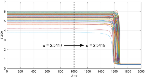
The constant parameters are given as ${r}_0=1.0$ , $L=10$ , $h=1.0$ , $a=0.1$ , $H=0.1$ , $\sigma =0.001$ . We solve the model (69) by using the Euler–Maruyama method.²⁵ Here, the time step width is $\Delta t=0.01$ , the number of steps is $T=1.0\times 1{0}^5$ , and the initial state ${z}_0$ is one of the stable equilibrium point of the state. We use the convergence value of the noiseless system with no input of (69) as the equilibrium point. With these settings and some random parameter ${\delta}_i$ , the bifurcation occurs when $c$ is at $2.5418$ (see Figure 4). Thus, we set $c=2.5417$ so that the network system is at a pre-deteriorating stage and satisfies Assumptions 1 and 2. The observation data for the sample covariance matrix are sampled from the calculation results of the numerical model at the interval of $T/N$ steps, where $N$ is the sample size. This calculation iterates $10$ times while changing the values of random noise. The system matrix $A$ is obtained by linearly approximating the model (69) in the neighborhood of the equilibrium point. The constraint on the input assignment $B$ is (51) with $m=2$ , that is, the number of input port is $2$ . In addition, we set ${\lambda}_{\mathrm{shift}}=0.05$ , which is used for design of the feedback gain.

4.3 Simulation results

Figure 5 shows the dominant eigenvector ${v}_1$ of the system matrix and the dominant eigenvector ${\tilde{v}}_1$ of the sample covariance matrix with the sample size $N=5$ and $N=100$ , respectively. According to Corollary 1, the optimal input assignment is ${B}^{\ast }=\left[{e}_6\kern0.3em {e}_7\right]$ since the 6th and 7th elements are the top 2 elements in absolute value of ${v}_1$ (see Figure 5A). In the case of ${\tilde{v}}_1$ with $N=5$ , the 6th and 7th elements are the top 2 elements in absolute value for 9 out of the 10 samples, while the 6th and 4th are the top 2 elements in absolute value for the rest one (see Figure 5B). Thus, the estimated optimal input assignment ${\tilde{B}}^{\ast }$ is equivalent to ${B}^{\ast }$ for 9 out of the 10 samples. Although ${\tilde{B}}^{\ast }=\left[{e}_6\kern0.3em {e}_4\right]\left(\ne {B}^{\ast}\right)$ for the rest one sample, it is also considered effective, because the 4th element has the 3rd largest absolute value in ${v}_1$ . In the case of ${\tilde{v}}_1$ with $N=100$ , the 6th and 7th elements are the top 2 elements in absolute value for all 10 samples (see Figure 5C), and then ${\tilde{B}}^{\ast }={B}^{\ast }$

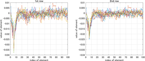
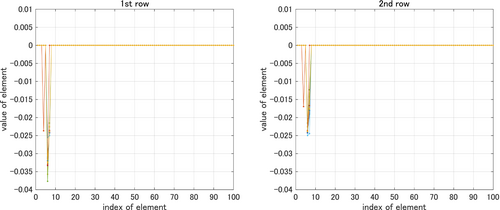
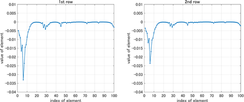
Figure 6 shows each row of the optimal feedback gain ${K}^{\ast }$ , which is obtained by using ${v}_1$ based on Corollary 1. Note that the feedback gain is a $2\times n$ matrix since the system has 2 inputs. Figure 7 shows each row of the estimated optimal feedback gain ${\tilde{K}}^{\ast }$ by using ${\tilde{v}}_1$ with the sample size $N=5$ for 10 samples. Figure 8 shows each row of the simplified feedback gain ${\tilde{K}}_s^{\ast }$ , which is obtained by setting all but the top 2 elements in absolute value to zero with respect to each row of ${\tilde{K}}^{\ast }$ with the sample size $N=5$ for 10 samples. Hence, each row of ${\tilde{K}}_s^{\ast }$ has only two non-zero elements. For 9 out of the 10 samples, the 6th and 7th elements are the non-zero elements in both rows of ${\tilde{K}}_s^{\ast }$ , that is, the indices of the non-zero elements are equivalent to the indices of the top 2 elements in absolute value of each row of ${K}^{\ast }$ . For the rest one sample, the 4th and 6th element are the non-zero in each row.

Figure 9 shows the dominant eigenvalue of the system matrix for four cases: just before bifurcation without any input, using the optimal state feedback with $\left({B}^{\ast },{K}^{\ast}\right)$ , using the estimated optimal state feedback with $\left({\tilde{B}}^{\ast },{\tilde{K}}^{\ast}\right)$ with the sample size $N=5$ for 10 samples, and using the simplified state feedback with $\left({\tilde{B}}^{\ast },{\tilde{K}}_s^{\ast}\right)$ with the sample size $N=5$ for 10 samples. In the case of using any state feedback, the dominant eigenvalue is shifted away from zero, that is, the system is re-stabilized. Note that, in the case of using the simplified state feedback, the dominant eigenvalue that is closest to zero corresponds to the case of using the sample with which ${\tilde{B}}^{\ast }=\left[{e}_6\kern0.3em {e}_4\right]$ .

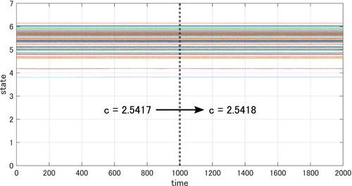
Figure 10 shows the state trajectory of the system with the simplified state feedback corresponding to the case where the dominant eigenvalue is closest to zero. Here, the bifurcation parameter $c$ slightly changes after $t=T\Delta t\left(=1000\right)$ . Even though $c$ changes, the equilibrium point does not change, that is, a bifurcation does not occur. Therefore, the network system is prevented from falling into a deteriorating stage.

From the above results, the simplified design method of the input assignment and feedback gain by using the dominant eigenvector of the sample covariance matrix is practically effective, although the change of the eigenvalues other than the dominant eigenvalue due to the simplification should be theoretically discussed.

5 CONCLUSIONS

In this article, we have proposed a method for designing the optimal input assignment and feedback gain for re-stabilizing an undirected network system based on pole placement under the condition that the system matrix is unknown and only HDLSS data of the state is available. The error evaluation of the simplification of the optimal design has also been presented. Furthermore, the numerical simulations have showed the effectiveness of the simplified design method.

This article assumes that the network of the system is undirected and the eigenvalues of the system matrix are distinct. Since a complex network system is not always undirected and the eigenvalues are not always distinct, we need to extend our method to the case where the network is directed and some eigenvalues are repeated. In addition, more detailed error analysis of the eigenvalue shift should be addressed.

CONFLICT OF INTEREST STATEMENT

The authors declare that they have no conflicts of interest.

FUNDING INFORMATION

This research was supported by The Moonshot Research and Development Program JPMJMS2021.

Open Research

DATA AVAILABILITY STATEMENT

The data that support the findings of this study are available from the corresponding author upon reasonable request.

REFERENCES

1Scheffer M, Carpenter SR, Lenton TM, et al. Anticipating critical transitions. Science. 2012; 338(6105): 344-348.
10.1126/science.1225244
CAS PubMed Web of Science® Google Scholar
2Chen S, O'Dea EB, Drake JM, Epureanu BI. Eigenvalues of the covariance matrix as early warning signals for critical transitions in ecological systems. Sci Rep. 2019; 9: 2572.
10.1038/s41598-019-38961-5
PubMed Web of Science® Google Scholar
3Scheffer M, Bascompte J, Brock WA, et al. Early-warning signals for critical transitions. Nature. 2009; 461: 53-59.
10.1038/nature08227
CAS PubMed Web of Science® Google Scholar
4Ghanavati G, Hines PDH, Lakoba TI, Cotilla-Sanchez E. Understanding early indicators of critical transitions in power systems from autocorrelation functions. IEEE Trans Circuits Syst I Regul Pap. 2014; 61(9): 2747-2760.
10.1109/TCSI.2014.2332246
Web of Science® Google Scholar
5Chen L, Liu R, Liu Z, Li M, Aihara K. Detecting early-warning signals for sudden deterioration of complex diseases by dynamical network biomarkers. Sci Rep. 2012; 2:342.
10.1038/srep00342
CAS PubMed Web of Science® Google Scholar
6Nakagawa T, Oku M, Aihara K. Early warning signals by dynamical network markers. Seisan-Kenkyu. 2016; 68(3): 271-274.
Google Scholar
7Matsumori T, Sakai H, Aihara K. Early-warning signals using dynamical network markers selected by covariance. Phys Rev E. 2019; 100:052303.
10.1103/PhysRevE.100.052303
CAS PubMed Web of Science® Google Scholar
8Oya S, Aihara K, Hirata Y. Forecasting abrupt changes in foreign exchange markets: method using dynamical network marker. New J Phys. 2014; 16(11):115015.
10.1088/1367-2630/16/11/115015
Google Scholar
9Kamal MAS, Oku M, Hayakawa T, Imura J, Aihara K. Early detection of a traffic flow breakdown in the freeway based on dynamical network markers. Int J Intell Transp Syst Res. 2020; 18: 422-435.
10.1007/s13177-019-00210-4
Web of Science® Google Scholar
10Fan J, Li R. Statistical challenges with high dimensionality: feature selection in knowledge discovery. Proceedings of the International Congress of Mathematicians, Vol. 3; 2006: 595-622.
Google Scholar
11Chernov A, Butakova M, Kostyukov A. Intelligent decision support for power grids using deep learning on small datasets. Proceedings of the 2020 2nd International Conference on Control Systems, Mathematical Modeling, Automation and Energy Efficiency (SUMMA); 2020: 958-962.
Google Scholar
12Yata K, Aoshima M. Intrinsic dimensionality estimation of high-dimension, low sample size data with D-asymptotics. Commun Stat Theory Methods. 2010; 39: 1511-1521.
10.1080/03610920903121999
Web of Science® Google Scholar
13Banno I, Azuma S, Ariizumi R, Asai T, Imura J. Data-driven estimation and maximization of controllability Gramians. Proceedings of the 2021 60th IEEE Conference on Decision and Control (CDC); 2021: 5053-5058.
Google Scholar
14Shen X, Morishita M, Imura J, Oku M, Aihara K. Low-sample-size data-driven re-stabilization of gene network systems. IFAC-PapersOnLine. 2022; 55(25): 241-246.
10.1016/j.ifacol.2022.09.353
Google Scholar
15Brauer A. Limits for the characteristic roots of a matrix. IV: applications to stochastic matrices. Duke Math J. 1952; 19: 75-91.
10.1215/S0012-7094-52-01910-8
Web of Science® Google Scholar
16Yasukata H, Morishita M, Shen X, Imura J. Single-input assignment design for stabilization of undirected networks towards ultra-early medical treatment. Proceedings of the 2022 European Control Conference (ECC); 2022: 1-6.
Google Scholar
17Lindmark G, Altafini C. Minimum energy control for complex networks. Sci Rep. 2016; 8:3188.
10.1038/s41598-018-21398-7
Web of Science® Google Scholar
18Varga A. A numerically reliable approach to robust pole assignment for descriptor systems. Future Gener Comput Syst. 2003; 19(7): 1221-1230.
10.1016/S0167-739X(03)00047-5
Web of Science® Google Scholar
19Ataei M, Enshaee A. Eigenvalue assignment by minimal state-feedback gain in LTI multivariable systems. Int J Control. 2011; 84(12): 1956-1964.
10.1080/00207179.2011.630026
Web of Science® Google Scholar
20Pandey A, Schmid R, Nguyen T. Performance survey of minimum gain exact pole placement methods. Proceedings of the 2015 European Control Conference (ECC); 2015: 1808-1812.
Google Scholar
21Oku M, Aihara K. On the covariance matrix of the stationary distribution of a noisy dynamical system. IEICE Nonlinear Theory Appl. 2018; 9(2): 166-184.
10.1587/nolta.9.166
Google Scholar
22Meister A, Li YH, Choi B, Wong WH. Learning a nonlinear dynamical system model of GENE regulation: a perturbed steady-STATE approach. Ann Appl Stat. 2013; 7(3): 1311-1333.
10.1214/13-AOAS645
Web of Science® Google Scholar
23Shen D, Shen H, Marron JS. A general framework for consistency of principal component analysis. J Mach Learn Res. 2016; 17(1): 5218-5251.
Google Scholar
24Watts D, Strogatz S. Collective dynamics of 'small-world' networks. Nature. 1998; 393: 440-442.
10.1038/30918
CAS PubMed Web of Science® Google Scholar
25Maruyama G. Continuous Markov processes and stochastic equations. Rend Circ Mat Palermo. 1955; 4: 48-90.
10.1007/BF02846028
Google Scholar

Volume33, Issue12

August 2023

Pages 6734-6753

Design of input assignment and feedback gain for re-stabilizing undirected networks with High-Dimension Low-Sample-Size data

Abstract

1 INTRODUCTION

2 PROBLEM DESCRIPTION

2.1 System description

2.2 Pre-deteriorating stage detection with HDLSS data

2.3 Design criterion

3 PROPOSED METHOD

3.1 Available information

3.2 Problem formulation

3.3 Optimal design with the dominant eigenvector of the system matrix

3.4 Error evaluation of the practical design

3.5 Proposed algorithm

4 NUMERICAL SIMULATIONS

4.1 Simulation model

4.2 Parameter setting

4.3 Simulation results

5 CONCLUSIONS

CONFLICT OF INTEREST STATEMENT

FUNDING INFORMATION

Open Research

DATA AVAILABILITY STATEMENT

REFERENCES

Figures

References

Information

About Wiley Online Library

Help & Support

Opportunities

Connect with Wiley

Design of input assignment and feedback gain for re-stabilizing undirected networks with High-Dimension Low-Sample-Size data

Abstract

1 INTRODUCTION

2 PROBLEM DESCRIPTION

2.1 System description

2.2 Pre-deteriorating stage detection with HDLSS data

2.3 Design criterion

3 PROPOSED METHOD

3.1 Available information

3.2 Problem formulation

3.3 Optimal design with the dominant eigenvector of the system matrix

3.4 Error evaluation of the practical design

3.5 Proposed algorithm

4 NUMERICAL SIMULATIONS

4.1 Simulation model

4.2 Parameter setting

4.3 Simulation results

5 CONCLUSIONS

CONFLICT OF INTEREST STATEMENT

FUNDING INFORMATION

Open Research

DATA AVAILABILITY STATEMENT

REFERENCES

Figures

References

Related

Information