1.1 Data

1.1.1 Population Data

The 2018 Colombian census offers a high-resolution population data set, consisting of counts of the de jure (usual) population across 551,028 enumeration areas. We obtained access to the coverage assessment conducted by the census ground teams, which enabled us to select 319,837 enumeration areas considered complete, that is, where at least 95% of the population was covered. The goal of this process was to establish a controlled environment with highly reliable population data. The coverage assessment also helped identify areas that were difficult to survey. We classified the complete enumeration areas based on the mean coverage rate of the municipality and settlement type they belonged to. Specifically, we categorized enumeration areas as ‘hard-to-reach’ if the mean coverage rate for their municipality and settlement type fell below the 10th quantile of the overall mean coverage rate distribution, corresponding to 69% coverage. For comparison, the national coverage rate for the 2018 census was 91.5%.

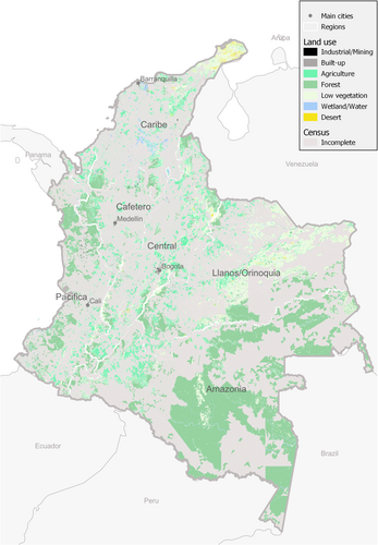
In addition to these data-access considerations, Colombia presents an interesting context for studying the relationship between population and satellite-imagery derived products because of its diverse environmental landscape, as depicted in Figure 1. Seventy-seven percent of its population is concentrated in urban areas, particularly in the largest cities of Bogotá (the capital), Medellín, Cali, and Barranquilla. The central region of Colombia, Central, which encompasses the Andean Mountain range and the highland plateau, has a relatively high population density. This is primarily due to factors such as fertile agricultural land, economic opportunities in cities like Bogotá, and historical settlement patterns. The northern coast of Colombia, Caribe, is another region with a significant population size. Cities like Barranquilla have a dense population due to their coastal location, ports, tourism, and economic activities such as trade and industry. The Pacific coast of Colombia, Pacifica, located in the west, has a lower population density compared to the Caribbean coast. The region is characterized by dense rainforests, challenging terrain, and limited infrastructure, which has hindered large-scale settlements. The eastern plains, Llanos/Orinoquia, have a lower population density compared to other regions. This vast grassland and savannah area is primarily used for agriculture, cattle ranching, and oil production. The southeastern part of Colombia, which includes the Amazon rainforest, has a relatively low population density. The area is largely covered by dense tropical rainforests and is home to indigenous communities. Access to this region is often challenging, limiting large-scale settlements and has therefore a lower proportion of enumeration areas completely covered by the census as shown by Figure 1.

1.1.2 Settlement Data

Early studies in population estimation from satellite imagery in data-scarce contexts relied on the manual digitization of building structures and rooftops, primarily using images from Digital Globe, for refugee settlements (Checchi et al. 2013), indigenous communities (Walker et al. 2014) and a city in Sierra Leone (Hillson et al. 2014, 2015, 2019). Advancements in computational power and machine learning systems for feature extraction, coupled with the increased availability of very high-resolution satellite images, have facilitated the automated production of countrywide settlement maps. Weber et al. (2018) leveraged this potential to estimate the population sizes in two Nigerian states from a sample of locations using satellite imagery to support vaccination campaign efforts. Due to the specialization of large institutes in settlement extraction models, subsequent years have seen a division between population modelers and settlement map producers. These include partnerships between Ecopia.AI and Maxar Technologies, the Joint Research Centre of the European Commission, the German Space Agency, Microsoft, and Google for the creation of new settlement layers.

The next generation of census-independent models has highlighted the valuable information contained in satellite-derived building footprints for population estimation from sampled locations (Boo et al. 2022; Darin et al. 2022; Dooley et al. 2021; WorldPop, & Institut National de la Statistique du Mali 2022; WorldPop, & National Population Commission of Nigeria 2021). All these models rely on a building footprint layer produced by Ecopia. AI & Maxar Technologies (2019). While a rasterized version of the layer was later made available covering the whole of sub-Saharan Africa (Dooley and Tatem 2020) the raw product is not openly available and no updates are planned for the foreseeable future. Other large-scale products are however openly available and regularly updated as described in Table 1.

Table 1. Settlement map attributes. The last column shows the percentage of missing enumeration areas per settlement type in Colombia with 4 the most remote and 1 the most urban.

	Attributes				Missing EAs per settlement type (%)
	Format	Resolution	Institution	Update	4	3	2	1
Land cover
Dynamic world	Raster	10 m	Private	Weekly	13	6	6	4
Built-up surface
Global human settlement layer	Raster	10 m	Public	5-year	11	2	0	0
Word Settlement footprint	Raster	90 m	Public	ad hoc	18	7	3	1
Building footprint
Microsoft	Polygon	50 cm	Private	ad hoc	15	8	4	1
Google	Polygon	50 cm	Private	ad hoc	24	11	7	5

Table 1 describes all the current openly available large-scale settlement maps and classifies them into three categories:

• 1.

  Building footprints: Building footprints are a polygon-based vector layer that automatically extracts the delineation of every building. There are two large scale and openly accessible building footprint layers:

• 1.

  The first one is produced by Microsoft using Bing Maps imagery with a spatial resolution ranging from 30 cm in dense area to 50 cm in sparse areas and a period ranging from 2014 to 2022 (Bing Maps Team 2022).

• 2.

  The second is produced by Google as part of their Open Buildings v3 release that uses Google Maps imagery with a spatial resolution of 50 cm. No specific imagery date year is provided (Sirko et al. 2021).

• 2.

  Built-up surface: Built-up surface layers are pixel-based raster data sets that map the distribution of the built-up surface. We assessed two global and openly accessible built-up surface layers.

• 1.

  The first one is the World Settlement Footprint produced by the German Space Agency using imagery from Sentinel-1 and Sentinel-2 that has a spatial resolution of 90 m and exists for two time points: 2015 and 2019 (Marconcini et al. 2021). The second one is the Global Human Settlement Layer produced by the Joint Research Center using the same imagery and with a spatial resolution of 10 m. They produced an additional product that focuses only on the residential area that we consider as a separate layer in this study. Those layers exist also at 100 m resolution for every 5 years between 1975 and 2020 with two additional forecasts for 2025 and 2030 (Pesaresi and Politis 2022).

• 3.

  Land cover map: Land cover layers are a pixel-based raster data sets that classify the Earth's surface based on the type of cover (e.g., urban, forest, agriculture). Because the power to predict population sizes is potentially hampered by the coarse land cover classes identified by these products, we focus on products with high temporal resolution to see if this can improves their value for prediction. We assess the Dynamic World layer produced by Google in partnership with the National Geographic Society and the World Resources Institute, using imagery from Sentinel-1 and Sentinel-2 that have a 10 m spatial resolution with a temporal resolution of every 2 to 5 days (Brown et al. 2022). We processed it as the mean value per pixel over the 2018 year.

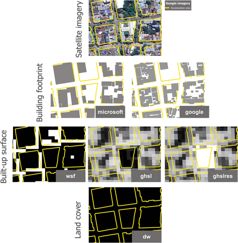
Figure 2 contrasts the six settlement maps to raw satellite imagery for several census blocks from the city of Neiva, Colombia. The main difference between them, as highlighted by the visual comparison, lies in their spatial resolution. To summarise settlement information for census enumeration areas, we used the count of building footprint centroids within each enumeration area and the proportion of each enumeration area covered by built-up surfaces.

2.1 Base Model: Hierarchical Bayesian Population Model

2.2 Base Model Calibrated With a Building Count Component

Directly integrating the $$\mathrm{settled\_area}$$ as an input data obfuscates the fact that the settled area is imperfectly detected from satellite imagery and therefore is not a direct observation. To link the satellite imagery products with observed information, we integrated an additional set of ground observations, the building count reported by the census team. The building count data from the census was used for model fitting, but was then considered missing for the model prediction stage to reproduce a data context where the only complete data available comes from satellite imagery.

2.3 Random Forest Model

We assessed how the performance of the process-driven probabilistic approach described above compared to that of a data-driven machine learning approach. We opted for the random forest framework (Breiman 2001) with the population density on the log scale as the response variable, in other words $$\mathrm{log}({{\rm{population}}}_{i}/{\rm{settled}}\_{{\rm{area}}}_{i})$$. Random forests have been shown to perform similarly to other machine learning/deep learning approaches in out-of-sample prediction when the observed units are small (Metzger et al. 2022). To study each settlement map, we varied the denominator (i.e., $${\mathrm{settled\_area}}_{i}$$) used to compute the population density while keeping the same selection of input covariates $$X$$ used in the base model of Section 2.3.1 as well as including the variables describing the region, department and settlement type. In this framework, we did not integrate the building counts observed by the census team because they were considered as only available for a sample of locations and random forest cannot accommodate missing data.

2.4 Model Evaluation

All models were trained within the R software (R Core Team 2022) using the Rstudio interface (Posit team 2023). To perform the Bayesian estimation of the model, we used the Stan software (Stan Development Team 2023) through the CmdStanR interface (Gabry and Češnovar 2023). We ran four Markov Chain Monte Carlo chains that included a burn-in period of 1500 iterations. We retained 1000 iterations following the burn-in period which were used for analysis. To assess model convergence, we used the default warning issuing from CmdStanR and checked that every parameter had an R-hat (the potential scale reduction factor, the weighted average of the between-chain and within-chain variances) below 1.1. To perform the random forest algorithm, we used the randomForest R package (Liaw and Wiener 2002) specifying 500 trees, a random sample of 2 covariates per tree (the number of covariates divided by three), and five observations for terminal nodes which correspond to the default settings in a regression framework.

To evaluate the performance of each model, we conducted out-of-sample cross-validation by comparing predicted population counts for all enumeration areas that were not sampled for model fitting. This allowed us to make claims about unseen areas and provides a more conservative estimate of model fit. In cases where the settlement map failed to identify any settled areas within the enumeration area, we interpreted this as equivalent to predicting zero people. We then summarized the performance with three statistics based on the percentage error such that errors in sparsely populated enumeration areas have the same importance as errors in densely populated enumeration areas. First, we looked at $${inaccuracy}$$ as measured by the median absolute percentage error (MAPE) to assess how close the predictions are in general to the truth. We then looked at the $${bias}$$ as measured by the median percentage error (MPE), to assess if the predictions systematically overestimate or underestimate. Finally, we looked at the $${imprecision}$$ as measured by the standard deviation of the percentage error to assess if the size of the prediction error varied a lot across enumeration areas.

To stress-test the performance of the population model, we summarized the performance of the three models for each of the six settlement maps across different contexts (six regions and three settlement types) when randomly sampling 1000 observations. For each combination of model and settlement map, we created 10 data sets by randomly sampling from the full-coverage census to assess the sensitivity of the modelling results to sampling variations.

3.1 The Bayesian Approach Performed Better With Less Informative Data

Figure 3 illustrates that building footprint layers consistently outperformed other settlement maps as the most reliable proxy for population sizes across all models and contexts, underscoring the importance of using settlement maps with the finest spatial resolution and specifically targeted at buildings. More precisely Google- and Microsoft-based models had a median inaccuracy of 41 and 43 people (i.e., 124% and 131% respectively) compared to 50 people (200%) for all the built-up surfaces. Conversely, the performance of Dynamic World, which covers all land cover types daily but lacks a specific focus on settlements, was consistently the weakest among all contexts and models (median inaccuracy of 62 people or 261%).

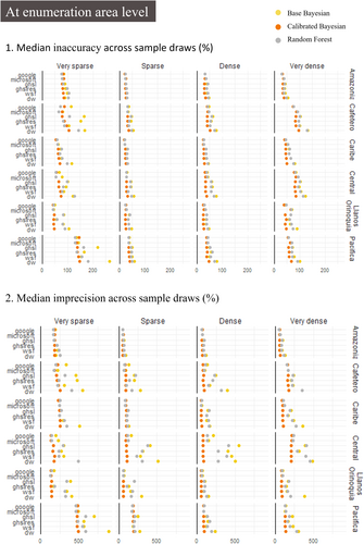
The comparison between modeling strategies highlights the advantage of the random forest approach for highly informative data sets but conversely the strengths of Bayesian modeling in contexts with limited information. In fact, for all settlement maps that were less detailed than building footprints, the calibrated Bayesian model outperformed the random forest model. By leveraging a sample of observed buildings, Bayesian modeling effectively converted the settlement map into building estimates, a quantity more closely related to population than settled area. Another notable strength lies in its ability to impose structural constraints, resulting in significantly less variation in prediction errors. Across settlement maps, the median imprecision of the calibrated Bayesian model was 91 people, while the random forest approach exhibited a higher median imprecision of 167 people. This difference suggests that the calibrated Bayesian model is less sensitive to extreme values in the sample.

3.2 The Bayesian Approach Performed Better With Biased Data

We looked at municipality prediction to see how well census-independent population models perform for larger spatial units. As expected, Figure 4 shows that aggregated population estimates were less prone to modelling error. The mean inaccuracy across all contexts, models and settlement maps dropped from 174% for enumeration area-level predictions to 40% for municipality-level predictions.

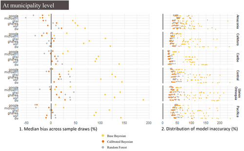
Assessing model performance for municipalities (i.e., aggregations of enumeration areas) revealed a prediction bias undetected at enumeration area level (see the left panel of Figure 4). Models using building footprints, particularly Microsoft, underestimated population counts for the municipalities situated in the region of Pacifica and Amazonia where population is less dense (Section 1.1) and enumeration areas without detected building footprints are more present (Table 1). The calibrated Bayesian model that utilized observed building count data better accounted for the under-detection of buildings with a median bias of −17% compared to −36% for the random forest model in the Amazonia region. The bias directly impacted on model performance at the municipality level. The best model was the calibrated Bayesian model for each of the settlement maps ranging from an average inaccuracy of 31% with the Global Human Settlement layer to 37% with Dynamic World. The distribution of the inaccuracy metrics across ten samples as displayed on the left panel of Figure 4 shows unexpectedly that the random-forest model did not lead to more variations between samples than the calibrated Bayesian model (a standard deviation of 10 percent point). A last insight from Figure 4 lies in the poor performance of the base Bayesian model that showed a median positive bias of 83% and inaccuracy of 95%.

3.3 Sparsely Populated Areas Were Harder to Predict

The municipality level assessment because of its larger size enabled us to account for the prediction bias seen in Figure 3 but obfuscated variation of prediction accuracy between settlement types. We thus created a custom municipality breakdown by settlement type by aggregating up the enumeration area predictions for which the census observations are complete per municipality and settlement type—a geographical scale that we named ‘medium scale’. The results presented in Figure 5 illustrate that across all models and settlement maps, prediction inaccuracy was greatest for very sparsely populated areas as shown by a mean inaccuracy of 50% compared to 29% for dense areas. This difficulty arises from the challenge in detecting remote settlements using satellite imagery products (Sanchez-Cespedes et al. 2024). The dense and very dense settlement types of all regions are the easiest to capture, except Central that contains the capital Bogotá. This may be due to higher heterogeneity in building occupancy across settlement types in the Central region with 72% residential buildings in very sparse areas and 87% in very dense areas according to the census. Generally, prediction inaccuracy is negatively correlated with the proportion of residential buildings (−0.21) and positively correlated with the standard deviation of the proportion of residential buildings (0.29).

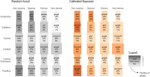
Revisiting the assessment of settlement maps, we see that the building footprint layers performed the best, with 34 of the 48 combinations of models and settings being more accurately predicted using the Google or Microsoft settlement map. This was especially the case when integrated within the random forest model where population counts were better predicted in 19 of the 24 settings with a building footprint layer (10 with Google and 9 with Microsoft). This result does not hold however in the remote Amazonia and Pacifica regions where, across models, the two layers had lower prediction accuracy than the built-up surface maps. Furthermore, the calibrated Bayesian model had better performances than the random forest one in 14 of the 24 settings, based on a mixture of settlement maps.

3.4 More Samples Decreased the Sensitivity to Sampling Errors

Settlement map-based population models are adopted in settings where ground data on population counts is hard to collect. It is therefore key to understand how increasing the sample size of ground truth data impacts on model performance.

Figure 6 shows how increasing the sample size from 500 to 10,000 enumeration areas had a small positive effect on the accuracy of the population model (from 224% to 202% inaccuracy at enumeration area level and from 44% to 33% at municipality level). This average accuracy increase was mainly led by the performance gain from the coarser settlement maps. The model that was the most impacted by greater sample size was the random forest model that saw enumeration area level prediction inaccuracy decrease by 31% points on average.

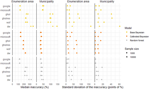
The greatest impact however of a larger sample size as depicted in the left panel of Figure 6, was the reduced variability of model performance across different sample draws, as indicated by the drop in the standard deviation of the inaccuracy metric computed for each of the 10 sample draws. Indeed, the standard deviation reduced by 96% points on average across all the combination of models and settlement maps at enumeration area level (32 percentage points at municipality level). Increasing the sample size thus reduces the sensitivity to sampling error and increases the consistency with which models reached the best prediction possible.

3.5 Population Estimates Were Less Accurate in Densely Forested Areas

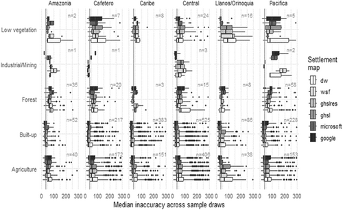
Figure 7 classifies the medium spatial scale units according to their main land use (Figure 1). It shows a trend that is common across the two population models: better performance was achieved in a built-up context than in rural areas. Because there are more spatial units in the built-up context (51%), change in accuracy will have a larger impact on countrywide accuracy assessment. The areas that were the most difficult to predict were by contrast the densely-forested areas of Amazonia and Pacifica.

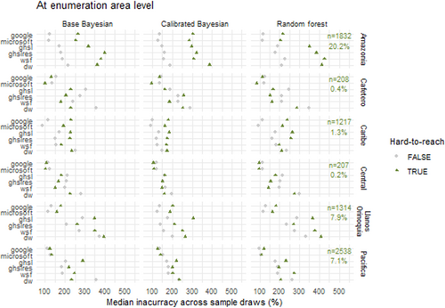
The last analysis assessed if population estimation can fill gaps where the census enumeration had the lowest coverage. On average, population prediction for accessible enumeration areas had an average inaccuracy of 56% when for inaccessible enumeration areas it reaches 91%. Figure 8 illustrates that the discrepancy is larger for coarse settlement maps (between 38% and 55% point difference) than for building footprint settlement maps (17 for Microsoft, 29 for Google). But the major difference is between regions: Figure 8 shows that in Amazonia the population hard to enumerate with traditional door-to-door collection methods is as challenging as for model-based estimation methods (186 percentage point difference).

4.1 The Importance of Building Counts for Estimating Population

The strong correlation between building counts and population sizes has fueled a recent surge of interest in harnessing satellite-derived settlement maps for population estimation. The initial endeavor to derive population figures from satellite images in data-scarce settings emerged in the context of temporary refugee settlements, relying on manual counts of visually identified building-like features (Checchi et al. 2013). Subsequent progress in computer vision and feature-extraction algorithms, coupled with increased spatial resolution of satellite imagery, led to the creation of large-scale automated settlement maps. While the past two decades have seen the global release of openly available built-up area maps as pixel-based representations of building coverage or settlement footprints (Marconcini et al. 2021; Pesaresi et al. 2013; Pesaresi and Politis 2022), the last 5 years have witnessed a proliferation of deep learning methods and computational power, enabling the extraction of built-up maps as polygon-based representations of building footprints (Bing Maps Team 2022; Ecopia.AI & Maxar Technologies 2019; Sirko et al. 2021). This wealth of information within building footprint maps has spurred the development of several population estimation models (Boo et al. 2022; Darin et al. 2022; Leasure et al. 2020; Metzger et al. 2022), and even a sub-Saharan Africa-wide interactive application to produce custom rapid response population estimates based on multiplying building counts by user-defined population ratios (Leasure et al. 2020).

Currently, openly available, large-scale building footprint products are offered by Google (Sirko et al. 2021), Microsoft (Bing Maps Team 2022) and OpenStreetMap (OpenStreetMap contributors 2023). However, the OpenStreetMap building layer has already been identified as problematic for country-wide mapping in data-scarce environments due to unequal coverage of manual mapping efforts (Chamberlain et al. 2024). Our study demonstrated that the other two building footprint layers, Google and Microsoft, tend to outperform pixel-based settlement maps across both model types. This aligns with Hillson's (2019) findings indicating that building counts are superior to rooftop area for population estimation as illustrated for the city of Bo in Sierra Leone. Continued improvements in open-source building detection from remote sensing therefore provides distinct advantages for population modeling.

However, we observed a systematic large negative bias in population estimation for two remote regions (Amazonia and Pacifica) using both building footprint layers. This highlights disparities in prediction accuracy in specific settings where settlements are harder to capture potentially due to less conventional housing structures or thicker forest cover, or in the case of Microsoft omitting to process areas considered as inhabited, and it challenges the notion of building footprints as the default settlement map for population estimation. Additionally, both data layers are produced by private companies with irregular and unpredictable open release timelines, while other producers, such as Ecopia AI, offer custom building footprint products commercially.

Nonetheless, our study demonstrates that in the absence of a reliable building footprint layer, leveraging building count observations collected on the ground enables the conversion of coarse settlement information into an estimate of building counts which results in higher accuracy of population estimates. This underscores the importance of integrating building listings into routine ground data collection during household surveys and making these building listings available to inform both population and building modeling. It is noteworthy that observed building counts do not need to originate from the same data source as observed population counts, highlighting the flexibility of the modeling framework. This finding aligns with the lessons learned from integrating social cartography in population estimation for settlements that are harder to detect in satellite imagery, such as indigenous communities (Sanchez-Cespedes et al. 2024). Finally, basing population models on the presence of settlements overlooks subpopulations that do not live-in buildings, such as the homeless or nomadic groups, which will lead to underestimation of the number people especially if those subgroups are clustered in space.

4.2 The Importance of Process-Driven Probabilistic Modelling in Data-Scarce Contexts

We have shown in this study that when the input data is complete, less biased, and detailed enough even off-the-shelf random forest models performed well. However, Bayesian probabilistic models performed better in contexts where the settlement layer is less informative because they can correct the bias. This is by extracting more information from coarser settlement maps by leveraging sparse information such as sampled building counts to increase the accuracy of the prediction model. All in all, when articulating different settlement maps for the various regional and settlement type settings as shown by Figure 5, the calibrated Bayesian model had slightly lower inaccuracy (31.4%) than the random forest approach (35.3%). The calibrated Bayesian model also demonstrated good properties in terms of precision of the population estimates with lower imprecision and better stability across sample draws than the random forest approach at the enumeration area and at the municipality levels.

This illustrates how specific challenges of scarce data settings may not be overcome by purely data-driven machine learning techniques as represented by the random forest approach, which is sensitive to sampling errors in small samples. Two features of the training sample are indeed driving machine learning performance: how large it is and how exchangeable with the prediction space it is. We conclude that in data sparse settings we cannot assume that the sampled training data is representative and unbiased and thus we need to develop probabilistic models that posit the structure of the underlying process of population spatial distribution. Another advantage of adopting a probabilistic model is its capacity to quantify the uncertainty within the modelled population estimates. To provide a relevant comparison with the machine learning model, however, we have only presented in this study point estimates from the Bayesian probabilistic models.

Thanks to the controlled environment provided by the Colombian census, we were able to systematically assess the bias and inaccuracy of each model by comparing estimates with the true enumerated population at different spatial scales. In practice satellite imagery-based population models are used when little is known about the true size of the population. In these settings we recommend the following steps to validate the outputs: (1) triangulating with external complete population data sources at coarser scale such as the World Population Prospect (United Nations Department of Economic and Social Affairs, Population Division 2024) to ensure large-scale validity, (2) triangulating with external partial population data sources at finer scale such as provided by the health and demographic surveillance systems (HDSS) (Herbst et al. 2021), and (3) the gold standard of out-of-sample cross-validation to assess prediction accuracy in contexts relevant to each use case (e.g. predictions into new regions, filling gaps between sample locations, prediction for new times).

4.3 A Demographic Data Revolution in Population Estimation?

The best performing model-settlement map combination, which paired the calibrated Bayesian model with the Google building footprint layer, achieved a median inaccuracy of 32% and a median bias of 1.5% at municipality level. This is a promising result in areas where no other data are available on population count. Our analysis has however highlighted the heterogeneity of the inaccuracy distribution. When decomposing the performance across subnational regions, we see that the median inaccuracy hides large disparity in the distribution of the prediction inaccuracy that ranges from 17% in Caribe in dense and sparse settings to 100% in the very sparsely settled areas of Pacifica which may be due to reduced accuracy of feature extraction algorithms for identifying buildings or built-up areas in densely forested areas (Muro et al. 2020; Sanchez-Cespedes et al. 2024). Similarly, the inaccuracy increased at finer spatial scales reaching a level of 148% for the same model combination. This study therefore illustrates the trade-off between spatial precision and reliability of the predictions, between densely and sparsely built environment and between high and low levels of mixed-use buildings.

Increasing the sample size of observations improves the precision of estimates, but has a smaller effect on their accuracy, highlighting the strong limitations of current models in relating satellite imagery-derived products to population counts using sparse survey data. To address these shortcomings, we suggest two pathways for improving accuracy across different settings and spatial scales. First, incorporating building occupancy types (e.g., residential, commercial, mixed, industrial) into the models could enhance the relationship between population and building counts, particularly in areas with many nonresidential buildings or high heterogeneity. Second, combining multiple settlement maps into a single model could improve performance by compensating for the shortcomings of individual data sources, addressing a key current challenge in demographic data revolution.