Numerical investigation of the Poisson's ratio of amorphous graphene sheets
Abstract
The one-atom-thick allotrope of graphite, C4 is called monolayer graphene and was discovered in 2004. It is well known for its fantastic electro-mechanical properties. While transverse contraction and Poisson's ratio were previously studied only for homogeneous or crystalline two-dimensional (2D) mono- and bilayer network structures under uniaxial tensile stress, we now numerically investigate these material properties for amorphous or non-crystalline monolayer graphene. Here, we pay special attention to the influence of the network heterogeneity. We find the stress-strain correlation in good agreement with the literature, and we find auxetic behavior, that is, negative Poisson's ratio, over a wide range within the elastic regime.
1 INTRODUCTION
In his pioneering work of 1932, Zachariasen published the Continuous Random Network (CRN) model as a two-dimensional (2D) cartoon model for bulk Silica glass [1]. Each Silicon atom is connected to three neighboring Oxygen atoms, forming sequences of corner-sharing triangles. A closed loop of n  -
- triangles forms an n ring, that is, a ring containing n members. The
  atoms link each of three randomly sized rings and, thus, form a network of randomly distributed n rings. If the network structure consists purely of six-rings and therefore looks like a flat honeycomb structure, we call it crystalline or homogeneous, in the case of a network of differently sized n-rings, as described above, we call it amorphous or heterogeneous.
Beyond  , the CRN model is well suited to describe the structure of many other flat materials which we include in the group of 2D materials. A 2D material that consists of only a single layer is called monolayer material. If it has two layers, we call it a bilayer. Up to 10 layers it is referred to as a few-layer material. Many groups reported on the production of 2D materials [2-4], as well as on their (opto-)electronic [5, 6] and mechanical properties [7-9], and, the dependence of the mechanical properties on structural defects [10, 11].
Graphene, the one-atom-thick allotrope of graphite, also belongs to the group of 2D materials. Its structure can be directly deduced from the CRN model by replacing all  atoms with C atoms and directly linking each to its three direct neighbors. Graphene has been isolated for the first time in 2004 by Novoselov et al. [12]. Since then, various studies have investigated its electronic and mechanical properties [13-15].
So far, several studies have been performed on Poisson's ratios (PR) for different crystalline structures. Gao and Xu [16] studied them for α-2D Silica (honeycomb structure, only six-rings). Gao et al. [17] found β-, γ- and δ-2D Silica, that is, three new, but still crystalline structures, and discovered large negative PRs (NPR) in ab initio tensile test simulations. Similar tensile tests with α- to γ-2D Silica, but using MD simulations, have been performed by Safaei et al. [18].
The influence of the network heterogeneity on the transversal strain and the PR of non-crystalline or amorphous 2D network structures has been investigated for mono- and bilayer 2D Silica by Stratmann et al. [19, 20]. Now, we numerically investigate transversal strain and PR with respect to the network heterogeneity of amorphous monolayer graphene.
2 METHODS
In our in-house tool JuMol [21], we simulate MD uniaxial tensile tests with monolayer graphene samples of five different network heterogeneities, 10 samples of each heterogeneity. The samples were generated using the Monte Carlo bond switching algorithm discussed by Bamer et al. [22].
Beginning with a crystalline sample that consists exclusively of rings of size  , a pair of directly bonded C4 triangles are randomly chosen and flipped. Hereby, the sizes of the adjacent rings change: two opposite rings decrease their sizes, while the two rings in between them increase their sizes by one.
 ) or groups of adjacent large rings (
 ), by means of the empirical law of Aboav [23]. Furthermore, we check if the bond switch brings the ring size variance σ of the network structure closer to a target ring size variance
  . The latter is the scaled ring size variance of an experimentally realized 2D Silica sample, measured by Lichtenstein et al. [24],
  :
:
 (1)
(1) [24].
[24].Only if both criteria are fulfilled, the bond switch is accepted. The potential energy is then minimized. This minimization step brings the network from a purely geometrically consistent (all atoms are fully coordinated, except those located next to the boundaries of the network) back to a physically meaningful structure.
Figure 1 depicts a network sample with heterogeneity of  after a comparatively low number of accepted bond switches. Many of the rings still maintained their original ring size of six shown in grey, while only a few changed their sizes to mostly five (green) or seven (blue), even fewer either decreased their sizes to four (green) or increased them to ring sizes beyond seven (magenta, cyan, and red). Note that larger rings have mostly small neighbored rings, as controlled by the law of Aboav [23].
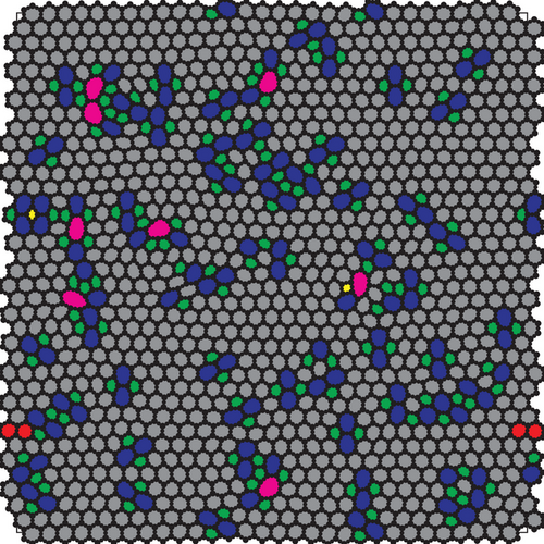
 . 2D, two-dimensional.
 (2)
(2) is a continuous value range around the discrete ring sizes given in Figure 2, for example,
  which is needed for a continuous envelope for the discrete ring size distribution. The value
  represents the mean ring size measured by Lichtenstein et al. [24] which is equal to six. The value σ is the ring size variance of the actual ring size distribution to be controlled. Since the depicted network sample already reached its target ring size variance, it is
  here.
here.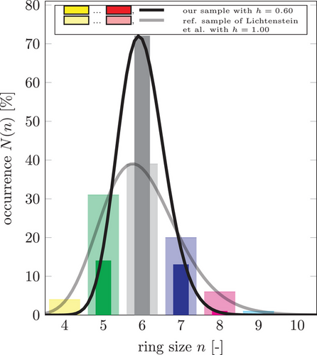
The wider and blurred bars in the background represent the ring size distribution of the reference sample, and the thick, gray line is their logarithmic envelope as given by Equation (2). The smaller ring size variance of the network sample shown in Figure 1, shows up in a much higher, and, much thinner peak of the black graph compared to the gray one.
If we perform many more acceptable bond switches on the network sample of  in Figure 1, we obtain the structure shown in Figure 3 with
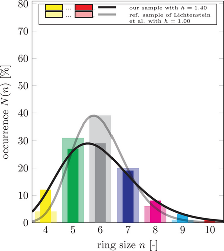
  . Figure 4 now tells us that more than 70% of all rings have changed their size, and the network has a larger number of smaller (
 ) and larger (
 ) rings than the reference sample. The corresponding peak of the logarithmic envelope (black) thus is slightly lower, and wider than that of the reference distribution (grey).
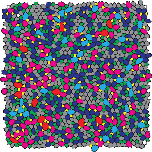
 . 2D, two-dimensional.
During the Monte Carlo bond switching algorithm, we use a pure 2D representation of the network structure. Before starting the actual deformation process, we introduce a small noise into the out-of-plane (z-) coordinate of every atom and relax the structure. Figure 5 shows that it forms bumps in z-direction, as they can be found in monolayer graphene.

 before start of the AQS deformation process. AQS, athermal quasistatic.
All samples are extended with a strain rate of  over 750 steps according to the athermal quasistatic (AQS) deformation protocol [22]. This protocol is defined by three consecutive steps: firstly, a box that contains all atoms is deformed affinely. In our case, the box is stretched in x-direction with a given x-strain rate while the y-length is kept fixed. In the second step, all atoms are displaced affinely, that is, according to their relative positions within the box. In our case, all atoms are only displaced in x-direction. In the third step, we minimize the potential energy of the network structure by adjusting the positions of all atoms in three dimensions with respect to their local field of potential energy. This step is necessary to transfer the artificially deformed structure back into its local basin of the potential energy landscape, that is, the non-affine displacements.
 (3)
(3) sums up all repulsion forces of each neighbor atom j in the repulsion potential
  and its attraction forces in the attraction potential
  , scaled by the bond order term
  . The latter takes into account if the connection between both atoms is a single, a double, or even a triple bond.
 ) is computed as
 (4)
(4) , and,
  . We, then, compute the Poisson's ratio as:
 (5)
(5) (
( ) averaged, over all N samples sharing the same heterogeneity. The sample averages will be denoted by a bar overhead,
  . The relation between a quantity
  and its sample average
  is given by
 (6)
(6)3 RESULTS
3.1 Sample averaged x-tensile stress  over sample averaged x-strain
Ebrahem et al. carried out numerical tensile tests to investigate the stress-strain correlation for amorphous graphene monolayers [27]. Figure 6 shows our numerically determined average tensile stress  over average tensile strain
  .
.
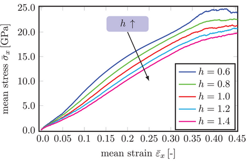
 over tensile x-strain
  , both averaged over five sets of each 10 of amorphous monolayer graphene samples with levels of network heterogeneity
  .
.The maximum tensile strength  is reached by the samples of the lowest heterogeneity
  at strain values of about
  and decreases with increasing heterogeneity h. This is in good agreement with the results of Ebrahem et al. [27]. At x-strain values exceeding 0.35, the graphs start losing their smoothness and begin to oscillate, which can be explained by first energy release events such as bond switches or isolated bond breaks.
3.2 Sample averaged y-strain  over sample averaged x-strain
In this section, we turn to the relation between average x- and y-strain shown in Figure 7.
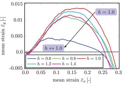
 over tensile strain
  , both averaged over five sets of 10 amorphous monolayer graphene samples with network heterogeneities
  .
.During deformation, the sample sets of all heterogeneities show both negative and positive y-strain, that is, contraction and expansion.
A very short period of transverse contraction in y-direction ( ) shows up within the range
  . We will have a closer look at the minimum transversal strains within this tensile strain range in Figure 8.
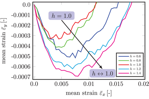
 .
.The samples of  reach the maximum value for the minimum transversal strain of
  . With both decreasing (
 ) and increasing network heterogeneity (
 ), the minimum transversal strain decreases to
  for the lowest network heterogeneity,
  , and to
  for the highest network heterogeneity,
  . We depict it by the black arrow in Figure 8.
Here and in the following, we will observe that the set of samples with  has an extreme value that becomes smaller or greater the farther the heterogeneity moves away to extreme values (
 ). Thus, we can state that network samples with
  are in a saturated state. Since they have the same ring size distribution as the reference sample realized by Lichtenstein et al. [24], one may refer to them as benchmark samples in the following and call the effect described above “benchmark sample saturation”.
For tensile strains between  , the samples enter the second, much longer period of transverse expansion (
 ). The largest transverse strain
  is achieved by the benchmark samples (
 ) and decreases, the farther the heterogeneity moves to extremal values.
Furthermore, Figure 7 shows a difference between the graphs regarding the lower ( ) and the larger heterogeneities (
 ). Whereas the three x-y-strain-graphs of the larger heterogeneities form a rather symmetric bow between both zero crossings and reach maximum transversal strains
  of around 0.15, the graphs of
  reach their maxima earlier. For further increasing x-strains up to
  , the graphs decrease with low curvature, forming a downwards-sloping plateau. For higher tensile strains, both slopes approach those of
  .
.
3.3 Sample averaged Poisson's ratio  over sample averaged x strain
Figure 9 shows the sample averaged PR in y-direction for tensile deformation in x-direction,  , over the sample averaged tensile strain in x-direction within the range
  . The light gray graph depicts the progress of the sample averaged PR, here exemplary visualized for
  . As all graphs oscillate heavily, we apply a Savitzky-Golay filter (sgf) with a window length of
  and a polynomial degree of
  to visualize the PR's dependency of the network heterogeneity. So, the five colored graphs in Figure 9 show the filtered, sample averaged PRs, denoted by
  , instead of
  .
.
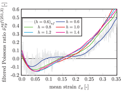
 for tensile strain
  , averaged over five sets of 10 amorphous monolayer graphene samples with levels of network heterogeneity
  , and filtered using sgf of degree
  with a window length of
  . sgf, Savitzky-Golay filter.
After having passed a minimum value below zero near  , the PRs of all five heterogeneities raise again to values greater than zero. Since they are the derivatives of the transversal strains with respect to the tensile strain, the difference between the lower (
 ) and the higher network heterogeneities (
 ) shows up here again: the graphs for
  make an S-shape and cross those of the higher heterogeneities. This phenomenon is especially pronounced for
  . Instead, the three graphs for
  raise by a slightly raising slope
  .
.
It is important to note that all five PRs exceed values of 0.5. This is no contradiction to classical mechanics because, for 2D materials, the upper limit of PR is 1.0 instead of 0.5, so  [28].
[28].
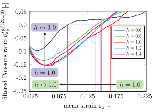
Figure 10 offers a closer look at the filtered, sample averaged PR within the tensile strain range of the auxetic behavior ( ). All samples of all heterogeneities show NPRs because they expand in y-direction while being stretched in x-direction. Considering the corresponding minimum values, we observe that the absolute minimum value is reached by the samples of
  with
with  at a tensile strain of
  .
.
 .
.Nevertheless, the minimum value for the benchmark samples ( ), is not much higher with
  , occurring at a tensile strain of
  . If we now assume that the slightly lower minimum PR of the samples with
  compared to the one of
  is due to some statistical fluctuations by taking into account the relatively low number of 10 samples per heterogeneity set, we can state that the minimum PR increases with h moving away from the value of the benchmark samples,
  , to either smaller (
 ) or greater values (
 ). And we conclude that the benchmark sample saturation shows up here again, highlighted by the blue arrow in Figure 10.
The zero crossings following the minimum PRs show this phenomenon at first glance: with the network heterogeneity moving away from  , the zero crossing of each graph shifts to lower tensile strains, with the absolute maximum at
  , and the minimum at
  . We visualize this phenomenon by the green arrow in Figure 10.
4 CONCLUSION AND OUTLOOK
As a groundwork for multiscale membrane modeling of electronic devices, we numerically investigate the influence of the network heterogeneity h on the transversal strain and PR of monolayer graphene samples under uniaxial tensile stress. We, therefore, perform molecular dynamics tensile test simulations with five groups of different network heterogeneities  , 10 samples in each group.
The stress-strain response that we obtain for each heterogeneity is in good agreement with the literature. All five sample sets reveal auxetic behavior, meaning positive transverse strains due to tensile loading, and, as a consequence, NPR. For the correlations of transverse strain and PR over tensile strain, the greatest or lowest extreme values are reached by the heterogeneity of  instead of the minimum (resp. maximum) one and shift to moderate values with h moving to either
  or
or  . Since the network samples with
  have the same ring size variance as an experimentally realized reference sample, we refer to these samples as benchmark samples and we name the phenomenon as benchmark sample saturation.
In all three correlations (stress, transversal strain, and PR over tensile strain), we observe that the graphs for the lower heterogeneities, namely  , are different than those of the higher heterogeneities,
  . This difference is worth being investigated further, together with the benchmark sample saturation.
ACKNOWLEDGMENTS
Open access funding enabled and organized by Projekt DEAL.


