Identification of creep parameters from multi-step relaxation tests on miniaturised specimen
Abstract
The small punch test (SPT) is a miniaturised method for thermo-mechanical materials testing. The combination of simple specimen geometry and low required specimen volume is ideal for minimally invasive characterisation and monitoring of the current material condition in technological systems, including nuclear plants.
The aim of the present study is to identify creep material properties of the chromium steel P91 (X10CrMoVNb9-1) via small punch testing. It is examined to which extent a single relaxation test is suitable to replace several creep tests at different force levels. The inverse parameter identification method utilises a non-linear optimisation approach in order to match the results of simulation and experiment. The simulation is performed using finite element analysis (FEA) and the considered material law aims to represent the high-temperature behaviour of steels. To this end, a modified Liu–Murakami model is specifically used along with linear elasticity and non-linear isotropic plasticity. We propose a strategy, that can be used to separately identify the Norton-parameters from multi-step relaxation tests performed on one specimen. Thereby, the applied strain (displacement, if utilising SPT) is kept constant after initial loading, which enables stress relaxation within the specimen. In case of the SPT, this behaviour yields a decreasing reaction force which approximately approaches a constant value. During the repeated loading phases, specimen failure may occur, due to further plastification of the specimen. Loading and relaxation cycles are repeated until specimen failure.
The identified parameters are validated via small punch creep experiments at different force levels. It will be shown that good agreement is observed when comparing the sets of identified parameters.
1 INTRODUCTION
The small punch test (SPT) as a miniaturised test method was developed around 1980 [1-3]. Its small sample volume makes it particularly attractive for applications in which the sample production is a significant cost factor, such as in nuclear power plant industry [4-6]. However, the benefit of the small sample volume and simple geometry comes at a cost. One disadvantage may be the inhomogeneous stress state, which makes material parameter determination difficult [7]. According to the current state of the art, numerous empirical correlations exist to determine material parameters from the measured values of the SPT such as yield strength, tensile strength and elongation at failure [8]. However, these correlations are generally material-dependent. To enable the identification of parameters of constitutive material laws, an inverse determination can be carried out [9]. In this case, the experiment is simulated and the material parameters used in the simulation are adjusted to reach the best agreement between simulation and measurement.
To perform a high-temperature relaxation test, the SPT-sample is firstly heated to a specific temperature. After reaching thermal equilibrium, it is loaded to a specific force or deflection. The deflection is then kept constant for a defined time period. If the specimen material exhibits viscoplastic properties such as creep, the force required to keep the displacement constant will decrease over time to a steady-state value. Typically, such a test is stopped after one relaxation, hence specimen failure does not occur. However, if the load is increased again, further local plastification occurs, accompanied by an increase in specimen deformation. This process can be repeated until specimen failure. This article deals with the question of whether several relaxation cycles can be simulated in succession and whether the data obtained from the experiments are sufficient to determine the creep parameters of the secondary creep stage separately.
2 TEST RIG AND EXPERIMENTAL RESULTS
The experiments were carried out on an SPT test rig developed at the IMFD [6], as shown in Figure 1. The sample loading was realised via a testing cylinder (1) mounted on a crosshead (2) which connects testing cylinder and loading rod (3). In this way, the specimen (4) can be loaded to a desired force. The target force for the multi-step relaxation test was  N. The sample was first inductively heated to
  °C. After the thermal equilibrium was reached, that is, no further thermally induced strains occurred in the test rig, the actual experiment was started. The target force was approached in a force-controlled manner. Then the piston displacement was stopped and fixed for
  h. After the time period had elapsed, the target force was approached again. The loading and relaxation cycles were repeated until specimen failure occurred. A total of three specimens (P1, P2, P3) were tested.
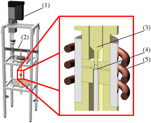
The specimens (diameter:  mm, thickness:
  mm) were manufactured from the remnant of a CT-specimen which was made of the creep-resistant chromium steel X10CrMoVNb 9-1 (P91).
During the small punch relaxation tests, several signals were recorded on which the inverse parameter identification strategy is based. The most important signals are: force (F), recorded at the upper end of the loading rod, and the specimen centre deflection (uM) at the bottom of the specimen. In addition, the temperature at the bottom of the sample was recorded. It served as the process variable for the temperature controller. To check whether the test rig reached thermal equilibrium, the temperature of the test rig was recorded at a large distance from the sample.
During specimen loading, the test rig deformed as well. In case of relaxation tests, this behaviour needs to be considered as the test rig released the accumulated stress upon specimen relaxation. This resulted in a small additional specimen deflection during the relaxation cycles until a state of equilibrium was reached. The stiffness of the test rig must, therefore, be taken into account in all simulations. Its determination was conducted experimentally by replacing the specimen with an carbide plate and logging the piston displacement along with the applied force. Taking into account the leverage effect of the crossbar, it was, thus, possible to calculate an equivalent stiffness c, which acts directly on the loading rod. To gain the best results possible, a non-linear stiffness was assumed.
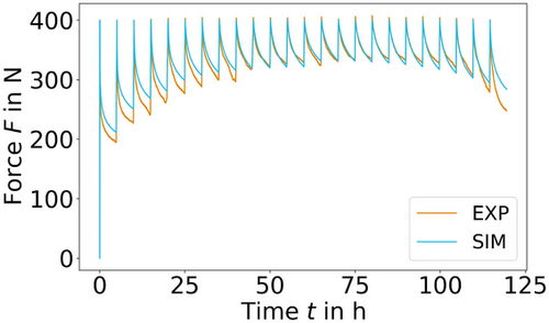
Figures 2 and 3 show the recorded measurement data of the experiments. In addition to the measured variables, an averaged curve was determined which is limited in time by the first sample failure. The repeatability of the experiments is excellent. The averaged curve served as the data basis for all simulations.
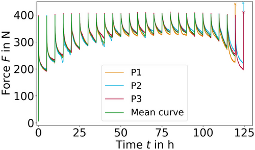
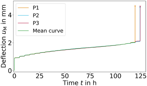
Due to the compliance of the test rig, the specimen deflection-rate during the relaxation cycle was non-zero ( ), as it would be required in an ideal relaxation test, where only the change in force is non-zero (
 ). In fact, the experiment presented here is a combination of a creep and a relaxation experiment. However, as explained later, this originally unintended behaviour holds the chance for a separate determination of the creep parameters of the secondary creep stage.
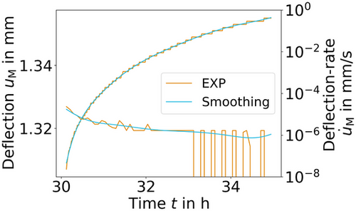
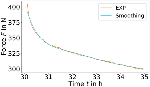
For the identification of the creep parameters, the determination of the deflection-rate was necessary as will be explained later on. The resolution of the displacement gauge of 1.0  m was not sufficient to produce a smooth time derivative of the recorded data as can be seen in Figure 4. The fluctuations in the force signal were also disadvantageous for an evaluation of the data. Therefore, the measurements of the specimen deflection and the reaction force were smoothed for each cycle with the help of splines. The spline curve was determined in each case using the function UnivariateSpline implemented in scipy.interpolate. The simple applicability and the direct access to its derivative were of great advantage. The use of splines was also a convenient approach, as in this way, one does not have to make any assumptions about the shape of the data set. When setting up the spline, it was important to adjust the order and the smoothing factor. The order was set to the highest value, 5. The smoothing factor was adjusted so that no overfitting occurred. The result of the successful smoothing is illustrated in Figure 4 for the specimen deflection and, in Figure 5, for the reaction force, each figure displaying the seventh cycle as an example. The numerical derivative in Figure 4 was created via finite differences with a massively increased step size to illustrate the advantage of splines. Reducing the step size would only worsen the numerical result.
3 CD-SPT-SIMULATIONS – CALIBRATION AND DISCUSSION
All simulations were carried out using the commercial software Abaqus V. 2022. The model was built axially symmetrical with the element type CAX4. Punch and die were assumed to be rigid bodies. The specimen was, thus, the only deformable body. The use of measurement data to construct the specimen geometry should be emphasised, for example, the specimen thickness and its diameter. The compliance effect of the test rig was taken into account by means of a connector element between punch and a rigid force-application-bar. The previously determined non-linear test rig stiffness c was assigned to the connector element.
 (1)
(1) . The material parameters for elasticity
  and plasticity
  were determined from uniaxial hot tensile tests and are given in Table 1.
 C: isotropic, linear elasticity and plasticity.
| E [GPa] | ν [-] | σ0 [MPa] | σ1 [MPa] | σ2 [MPa] | a [-] | εg [-] | d [-] |
|---|---|---|---|---|---|---|---|
| 159.0 | 0.315 | 210.663 | 379.395 | 43.885 | 555.820 | 12.024e-3 | 3.323 |
 (2)
(2) (3)
(3) (4)
(4) (5)
(5) and
and  are the rupture-stress and the equivalent stress, respectively, σ1 is the first principle stress,
  is the deviatoric stress tensor. ω denotes the damage variable which evolves from zero to the fully damaged state. To avoid numerical difficulties, ω is capped above
  [11]. The Liu–Murakami model is stated here in its uniaxial form, since only the uniaxial form can be implemented in the Abaqus user subroutine CREEP. The model was further modified to account for creep-strain-hardening which offers the possibility to represent primary creep as well [12]. B1 controls the impact of primary creep, while k describes how fast steady state creep is reached. Furthermore, it is important to group the parameters which affect certain creep regimes. Secondary creep is only influenced by
  and the Norton exponent n. The primary creep regime is described by B1 and k, while the tertiary creep regime is affected by the remaining parameters M, q2, χ and α.
 ,
,
 (6)
(6) and
and  of the simulation and experiment, respectively.
  denotes the vector of material parameters, which were used in the material model. The error to be minimised can be represented as the squared norm of the residuals
  . The weights
  can be adjusted so that, on the one hand, the variance of the residuals is taken into account and, on the other hand, that residuals with a low confidence level are weighted lower than residuals with a high confidence level.
In the present optimisation problem, the total residual  was composed of several data sources. On one hand, an error resulted from the force/time curve and on the other hand, from the deflection/time curve. Furthermore, the total residual was extended by a penalty term, which denotes the time deviation of the last increment of the simulation from the experimental specimen failure time. Using this method, it can be ensured that material parameters are calculated in a way that the simulation runs at least through all compared relaxation cycles.
 can, thus, be defined logarithmically equidistant in the time range
  .
.  denotes the beginning of the relaxation and
  the beginning of the following loading phase. After the residuum was calculated for each cycle, a single vector was assembled:
 (7)
(7) (8)
(8) (9)
(9) (10)
(10) and
and  , they are logarithmised to achieve faster identification.
 on the difference between the maximal time points of simulation and experiment
 (11)
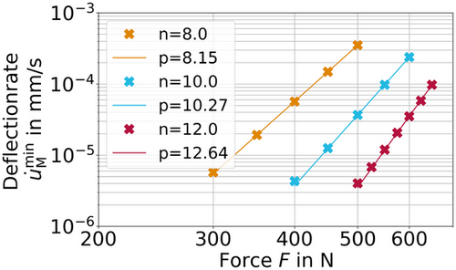
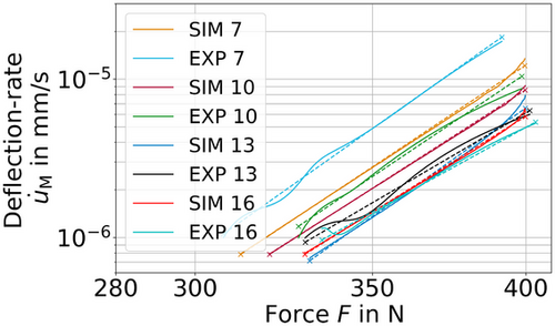
(11)It is not advisable to identify all parameters at once. To account for a priori knowledge about the sensitivity of the parameters in certain creep regimes, one should split the identification. First, the secondary creep regime shall be identified, where only data are used which lies inside the time interval  . Due to the strong correlation of the creep parameters, for example, B and n, a simultaneous determination is not advisable as well. An alternative method shall be tested in the following. In the literature on high-temperature SPT research, many methods are presented to convert both the reaction force into a uniaxial equivalent stress and the deflection-rate into a uniaxial equivalent strain-rate [13-15]. The determination of the parameters is not always clearly derived and usually depends on material, temperature and/or other state variables. However, a common feature is that the slope of the double log strain-rate/stress relationship from uniaxial creep tests corresponds to the slope of the deflection-rate/force relationship from SPT-CF investigations [16, 17]. Therefore, to support this hypothesis, several SPT creep simulations, with primary and tertiary creep turned off, were performed at different loads and Norton exponents. Subsequently, linear regression was used to determine the minimal deflection-rate of the secondary SPT creep regime. Using the pairs of deflection-rate and force values, Figure 6 was generated.
 (12)
(12) was confirmed for all tested Norton exponents
  . The crosses in Figure 6 correspond to the simulations and the solid lines to the non-linear regressions according to Equation (12). The maximum relative deviation between the exponents is 5.3%.
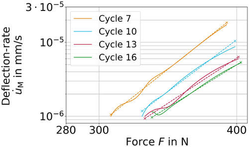
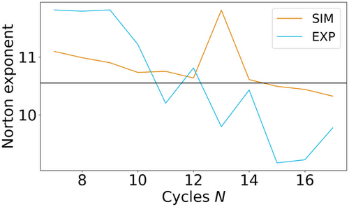
Having the hypothesis supported, the identification procedure for the parameter p was now applied to the relaxation cycles 7 through 17 (see previously defined time interval) of the multi-step relaxation test. The mean value of the identified exponents is  . Figure 7 shows the regressions for cycles 7, 10, 13 and 16. The approximately linear relationship was an important indication of the applicability of the Norton power law and therefore of the importance of the secondary creep regime. The Norton exponent is, thus, considered to be identified. Consequently, B remained the only parameter left for the determination of the secondary creep regime parameter set. Using non-linear optimisation and an error definition comprising the cycles 7 through 17 cycles (Equations (7-11)), the parameter B was identified, see Table 2. For the given material law, these parameters have been identified separately and from only one experiment.
| B0 [MPa] | B1 [MPa] | k [-] | n [-] | M [-] | q2 [-] | χ [-] | α [-] |
|---|---|---|---|---|---|---|---|
| 557.35 | 91.57 | 7.17 | 10.55 | 2.74e-16 | 3.78 | 2.11 | 0.24 |
The remaining parameters are for the creep regimes I and III. Primary creep is processed first, followed by creep-damage. To not influence the result of the previously identified parameter B, only B1 and k were optimised from the primary creep parameter set while  . For this optimisation, the data of cycles 1 through 6 were used. Afterwards, the remaining parameters were identified using the data of the cycles 18 through 24, see Table 2.
Good agreement can be seen in the force/time curve, see Figure 8 as well as in the deflection/time curve, see Figure 9. However, even with primary and tertiary creep, it is not possible to map the force/time curve perfectly. If the influence of primary creep would be increased, the force/time response of the first cycles would improve but this would simultaneously lead to an increase in deflection in all cycles. Meaning, to improve the force/time curve, one must worsen the whole deflection/time curve. The same principle applies to the tertiary stage. With our current test rig, it was not possible to measure the thickness reduction of the specimen centre accurately. Having this measurement, it would be possible to estimate the friction coefficient which has a huge impact on the results and therefore on the identified parameters [6, 18, 19]. The friction coefficient was assumed with  , which is often used in literature [6, 20].
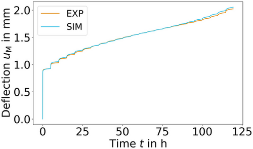
The procedure, which was used for identifying the Norton exponent, can of course be applied to the simulation as well, see Figure 10. The current working hypothesis states that the slope of the deflection-rate/force curve can be used to approximate the Norton exponent. From Figure 11, it is apparent that the hypothesis is missing an ingredient which is currently still unknown. The negative slope indicates that the parameter p depends on some evolving quantity, which is already included in the simulation model since both simulation and experiment show this behaviour, for example, the plastic strain, the creep strain or the global specimen deflection. Since the slope of the deflection-rate/force curve for one exemplary cycle does not vary, while the central deflection and creep strain does, in fact, evolve, it is near to rule them both out and consider the plastic strain as the more likely choice. However, the plastic strain as a field quantity is not straightforward to include in a global value like the Norton exponent. This makes more research on this topic necessary and motivates future work.
The validation of the identified material parameters involved three different forces ( N) with three specimens for each force. The specimens were heated to
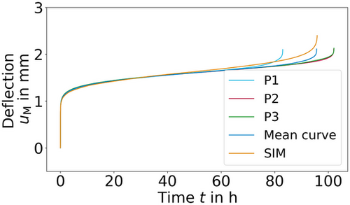
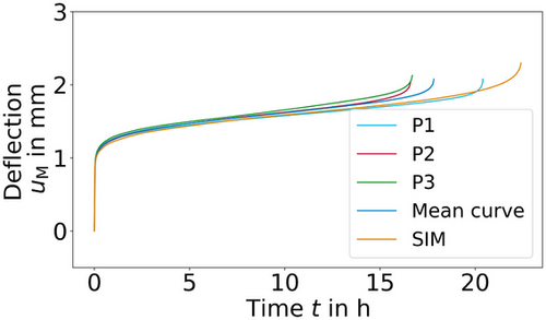
  C. Material from the same batch was used for the creep tests. The results are shown in Figures 12-14. Here, clearly, the second stage is mapped very well. Considering the typical scatter of creep experiments, the specimen failure time is also represented very well. However, differences for the secondary creep stage of Figure 12, displaying the creep experiment at
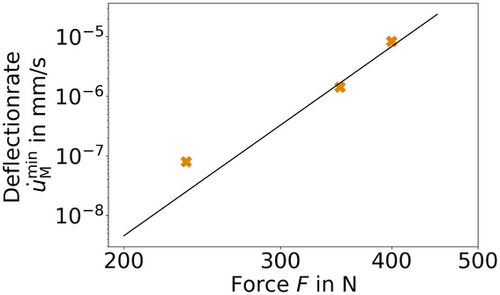
  N, are observed. The reason for this could be a change in the parameters due to a change in the creep mechanism. This assumption becomes more likely considering Figure 15. Crosses represent the experiments and the line represents a power–law curve with the previously identified Norton exponent. Only the experiments at
  N and
N and  N are mapped well. From this, we can conclude that the Norton exponent is indeed dependent on the applied load [21, 22].
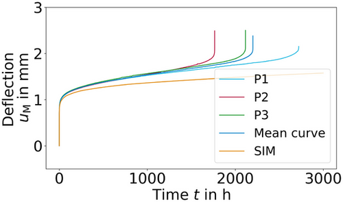
 N and a simulation using the previously identified parameters.
 N and a simulation using the previously identified parameters.
 N and a simulation using the previously identified parameters.
4 CONCLUSIONS
- The relaxation tests, carried out at only one force and one temperature, are suitable for the separate identification of secondary creep parameters.
- The repeatability of relaxation tests is significantly better compared to creep tests.
- The identification of creep parameters for the secondary stage requires the performance of several relaxation cycles, as the influence of primary creep is significant in the first cycles.
- The parameters determined with the proposed identification strategy could be successfully validated on CF-SPT creep tests.
ACKNOWLEDGMENTS
The financial support of GRS gGmbH (Society for Plant and Reactor Safety) projects (funding code 1501578) by the Bundesministerium für Umwelt, Naturschutz, nukleare Sicherheit und Verbraucherschutz (BMUV) is gratefully acknowledged. The authors appreciate the scientific collaboration with Dr. Petr Dymáček from the Institute of Physics of Materials of the Czech Academy of Sciences and Dr. Eberhard Altstadt, Head of the Construction Materials Department, Institute of Resource Ecology at the Helmholtz Centre Dresden-Rossendorf. Furthermore, the authors thank the technical staff who made a significant contribution to the sample preparation and experimental procedures.
Open access funding enabled and organized by Projekt DEAL.


