A volumetric heat source model for the approximation of the melting pool in laser beam welding

1 INTRODUCTION

As a versatile process, laser beam welding minimizes thermal distortions by creating a small heat affected zone. It is a highly efficient procedure for joining metals, which is used in various industrial sectors. An important aspect of the welding process is the so called mushy zone. This zone creates the transition area between molten and solid material during the welding process. An accurate characterization and identification of the mushy zone is of great importance to understand the material behavior and the formation of solidification cracks. The analysis of the mushy zone regarding the stress and strain distribution enables better adjustment possibilities of the welding parameters. This allows defects such as cracks and pores to be prevented and the quality of welded joints to be improved. Moreover, the analysis of the mushy zone provides valuable insights for advancing welding techniques and optimizing industrial welding processes. In order to achieve such enhancements, two heat source models will be discussed below. The first model is developed by the “Bundesanstalt für Materialforschung und -prüfung” that represents an equivalent heat source model, compare [1] and [2]. This means that an isotherm is reconstructed from prior Computational Fluid Dynamics (CFD) simulations using Lamé curves and transferred into the simulation through Dirichlet boundary conditions. The geometry of the isotherms corresponds to that of the melt pool and is approximated based on a previous CFD simulation. The second model is a modified model based on a conical heat source model. The conical model is common for laser beam welding processes and is described by a Gaussian distribution, for more information, see refs. [3-6]. When it comes to the modifications, a range of assumptions are made, encompassing the neglect of the Gaussian distribution as well as the disregard for thermal conductivity. This contribution deals with the numerical implementation of the two named heat source models and analyzes the resulting temperature distributions. Therefore, in Chapter 2 the thermomechanical model is presented. The overall equations are introduced and the representation of the heat dissipation is shown. After that, the heat source models are discussed in Chapter 3. The model based on Lamé curves is briefly explained. The main focus is on the conical model and its modification regarding the change in energy input. Chapter 4 deals with the numerical examples are depicted with the boundary value problem and the resulting outcomes. Finally, in Chapter 5, all the results are summarized and an outlook is provided.

2 THERMOELASTIC FORMULATIONS

Within this contribution, thermomechanical material behavior is considered. Therefore, the numerical description of the laser beam welding process is based on the balance equations:

(1)

Within the above equations, the Cauchy stresses are given by σ, the body forces are given by f, the density by ρ, the heat source by r, the heat flux by q, the current temperature by θ, the free energy by ψ and the strains by ε. The free energy equation

(2)

taken from ref. [7], is used in its volume specific formulation. Therefore, one defines . If one takes the derivative of the free energy with respect to strains and temperatures, one finally obtains

(3)

from Equation (1.2). In Equations (2) and (3), κ describes the bulk modulus, μ the shear modulus, c the heat capacity, θ₀ the initial temperature and the coefficient of thermal expansion. In order to perform simulations, a thermomechanical finite element model is generated which takes into account the above equations and assumptions. A small strain formulation with linear hexahedral volume elements are used. Furthermore, the model needs to represent the heat loss across the surfaces. For this purpose, surface elements are added based on the finite element mesh connectivity in a separate MATLAB code. These surface elements utilize the same nodes as the outer volume elements and are also linear. The heat loss is based on the equation 

(4)

and takes into account both heat convection and thermal radiation. Here, q defines the heat flux vector, the heat transfer coefficient for convection, the ambient temperature, the Stefan-Boltzmann constant with a value of approximately and the emissivity.

3 HEAT SOURCE MODELS AND THEIR NUMERICAL IMPLEMENTATION

In the following chapter, the two heat source models will be discussed. On one hand, a model based on isotherms, see refs. [1] and [2], and on the other hand, a modified conical model representing a volumetric heat source. Although both models are based on the data from a previous CFD simulation, the heat input is applied in different ways, namely through Dirichlet boundary conditions or body forces. Therefore, the two models will be presented in more detail regarding their numerical implementation and specific characteristics. This will allow a precise evaluation of the results of the welding simulation afterwards.

3.1 Lamé curve model

The model based on Lamé curves (isotherms) serves as a reference solution in this paper. Originally, it was developed by the Bundesanstalt für Materialforschung und -prüfung (BAM) and represents the weld pool geometry of laser beam welding processes. This geometry is obtained from a prior CFD simulation which provides a detailed model of the melting process and the associated effects. This includes fluid flow, reflection, partial material vaporization and the associated keyhole phenomenon that typically occurs during depth welding. The specific molten pool geometry is then transferred to a finite element simulation using multiple data points, as shown in Figure 1, which describe the isotherm of the liquidus temperature . The liquidus temperature is the threshold temperature above which no solid phase exists anymore. Between and the solidus temperature , there may still be solid particles present in the material. This temperature range defines the mentioned mushy zone. A detailed description of the effects in the completely molten region is outside the scope which is the reason why it is modeled by a constant temperature equal to . 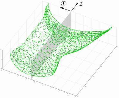The data of the CFD simulation is provided by the BAM. 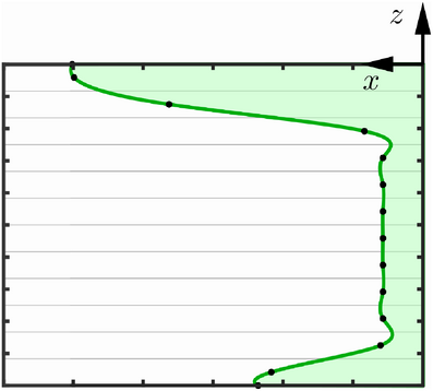The processed temperature field from the CFD simulation of the isotherm is represented in a point cloud and subsequently divided into different layers along the thickness direction (z-axis) within the range and . The coordinates of the points within each layer are then examined to obtain maximum and minimum values in each axis direction (x- and y-direction). These values then define the radii a and of an ellipse, which is positioned at the center of each layer at . The radius a in y-direction only changes along the height, while the radii in the x-direction vary with respect to both the height and the position relative to the center of the ellipse. In the front part, the radius is used, while in the rear part, the radius is utilized, which is why i can stand for f (front) or r (rear). This process is repeated for any desired number of layers, resulting in multiple defined ellipses. Finally, the individual values are connected using cubic spline interpolation, resulting in a geometry similar to the one shown in Figure 2. By employing cubic spline interpolation along the height, the radii of the ellipses at any given z-value can be interpolated. Lastly, the ellipses geometry is used to query the mesh nodes. For each node, it is checked whether it lies inside or outside the geometry. This is done using

(5)

If a node is found to be inside or exactly on the ellipse (i.e., the interpolated isotherm), the liquidus temperature is assigned to it as a Dirichlet boundary condition. Thus, an approximation of the molten pool geometry from the CFD simulation is obtained.

3.2 Conical heat source model and its modification

The second heat source model is a modified version of the standard conical heat source model, see refs. [5] and [6]. The conical model is based on a Gaussian distribution, see Figure 3, and its heat source is defined by

(6)

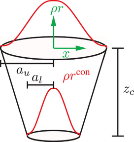
where denotes the volumetric heat flow density, the maximum value of volumetric heat flow density at , x, y and z the coordinates in 3D, a the radius of the conus variable over the height, the upper radius, the lower radius and the height of the conus. The parameter f is used to adjust at the outer edge of the cone,that is, for . For example, for , the density for is reduced to only five percent. With these two equations one can calculate the volumetric heat flow density for every point inside the geometry. Furthermore, when using this model, both the solid and liquid phases, including their respective material behaviors, should be taken into account. This allows for the consideration of effects such as latent heat, which have an impact on the temperature evolution. However, when applying this model, there is a continuous input of energy, leading to a temperature increase that significantly exceeds . Nevertheless, the region above , representing the purely liquid phase, is not necessarily essential for further investigations. Instead, the focus lies on the mushy zone, which is situated between and , and its microstructure. Therefore, it is considered meaningful to limit the temperature within the melting pool to a range around , similar to the Lamé curves model. While temperature peaks above still occur within the melting pool, the material behavior is approximated for the liquid phase in this case, neglecting some of the physical effects present in the melt. Consequently, a modified heat source model is developed, wherein the energy input is adjusted so that the temperature does not significantly exceed the desired limit of . This energy or heat input is defined to describe the volumetric power density associated to the laser while the Gaussian distribution is neglected. Additionally, for the following estimation, it is assumed that becomes negligibly small and that a constant temperature exists in the melt pool, resulting in becoming zero. Therefore, it follows from Equation (3) for the estimation of the modified energy input

(7)

With the help of Equation (7) and taking into account the approximation , the temperature can be estimated to

(8)

Now, it is assumed that the temperature in the system is initially raised with for a specified number of time steps , so that holds. Here, is a selected deviation from . If is met, the further energy input is estimated using Equation (7) by solving for . For this estimation, is approximated as and it is stated that the energy input cannot become negative. The physical limit, , cannot be exceeded. It follows

(9)

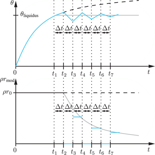
In summary, the temperature is initially raised using until a specific threshold, , is reached. If this threshold is exceeded by estimating the temperature in the subsequent time step, the condition from Equation (9) comes into play for further determination of the energy input. This approach aims to set a temperature within the range around throughout the entire heat source. This process is visualized in Figure 4. Note that in contrast to the Lamé curve model, the geometry of the isotherm is not taken from CFD simulations, but a conical region of the melting pool is assumed, which is artificial. This is especially important for the results in Chapter 4.2.

4 NUMERICAL EXAMPLES

In order to compare the two discussed heat source models this chapter deals with the numerical examples. First the boundary value problem and the necessary material and process parameters are presented. After that the results regarding both models are depicted and analyzed. All calculations are carried out with the Finite Element Analysis Program (FEAP), see ref. [8].

4.1 Boundary value problem

For the numerical realization of the laser beam welding process a suitable boundary value problem is defined. Therefore, a boundary value problem similar to the conducted experiments by BAM has been chosen. To keep the computational time low, only a small portion of an experimental setup is simulated. Figure 5 schematically illustrates the experimental setup. It involves the use of a thin plate made of austenitic chrome-nickel steel with a thickness h of 1 mm, a length 3l of and a width of . The plate is clamped at one edge. The simulated section, highlighted in blue in Figure 5, is magnified and shown in Figure 6. Here, the section has a thickness h of 1 mm and a length l and the width b of and , respectively. Similar to the overall plate, this segment is statically supported and clamped at , see Figure 6. Regarding the thermal boundary conditions, implemented as Robin boundary conditions, see ref. [9] and adapted from ref. [10], the surface elements discussed in Chapter 2 are used at the top and bottom of the system, namely and , respectively. These surface elements describe the heat dissipation and have a heat transfer coefficient of and an emissivity of 0.85. Due to the relatively small surface area, the vertical edges of the system are simulated without heat dissipation.

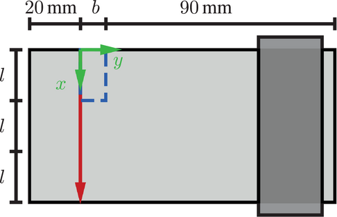
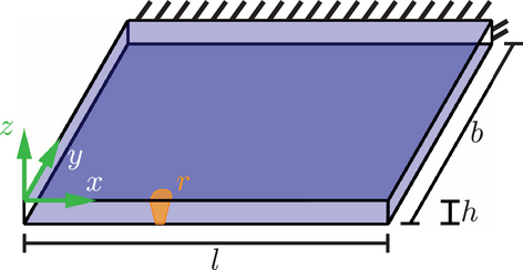
The system is discretized by linear hexahedral elements and 60 × 30 linear rectangular surface elements each for the upper and lower surface. This leads to 44 286 degrees of freedom. Furthermore, a time step size of is used. An austenitic chrome-nickel steel (1.4301) is used. The chemical composition of the steel can be found in Table 1.

TABLE 1. Chemical composition of the used austenitic chrome-nickel steel 1.4301.

Element:	C	Si	Mn	P	S	Cr	N	Ni	Fe
wt%:	0.02	0.41	1.6	0.028	<0.002	19.09	0.095	8.06	69.9

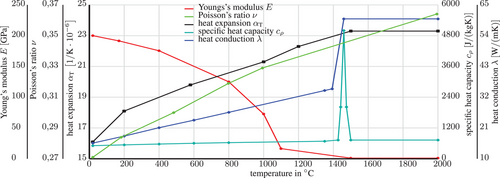
The data is provided by the BAM. The material parameters are adopted from the BAM. They are obtained from the software Sysweld and presented graphically in Figure 7. Since no data is available for the density of the material, it is assumed to remain constant with temperature and is set to a value of . This value is taken from ref. [11] and corresponds to the density at . As indicated by the data points in Figure 7, the material parameters are provided only for certain temperatures. However, it is necessary to consider the intermediate temperature ranges as well. Therefore, a linear interpolation of the values is performed using

(10)

This applies to the entire temperature range from to . In the equation, and represent the temperatures with the known parameters and . To determine the parameter p for an intermediate temperature θ, Equation (10) is applied. Moreover, a welding velocity of is chosen. The energy rate (power) for the modified volumetric heat source model, that is, , has a value of and the temperature used in the Lamé curve model corresponds to the liquidus temperature of .

4.2 Results

Since the geometry of the melting pool described by the two models here is different, see Chapter 3, the results presented are assumed to differ. The aim is the description of the melting pool and a qualitative investigation of the temperature field in the surrounding region. In Figure 8, the results using Lamé curves are presented. In all time steps, it is evident that a constant temperature of 1500° C, corresponding to the liquidus temperature, exists within the melt pool. Additionally, in the first two time steps, the geometry of the melt pool is clearly visible. Both the characteristic depression in the front part of the heat source and the elliptical shape in the longitudinal section are apparent. Furthermore, a strong temperature gradient forms in the front region of the heat source as well as to its sides and rear, where the mushy zone builds up.

The results for the modified model exhibit similar behavior. It is worth mentioning that the radius of the black cylinder in Figure 9 corresponds to the upper radius of the conical heat source used and is only added to the illustration for identification of the melting pool region. This is intended to demonstrate the behavior of temperature within the heat source. The goal is to achieve an approximately constant temperature distribution. Starting with the interior of the volumetric heat source, it is apparent that despite a continuous energy input and significantly reduced thermal conductivity, a temperature gradient can be observed in the front region. This gradient could be explained by the heat dissipation from the source. In the rear part, however, a constant temperature is formed. Especially at the locations where a significant color difference occurs due to the scale, the conical shape of the heat source can be discerned, with a larger radius at the top and a smaller radius at the bottom. In the rear part, the typical temperature tail is evident.

5 CONCLUSION

The present paper discusses two heat source models for the description of the resulting temperature field in laser beam welding processes. They essentially differ in their numerical realization: The Lamé curve model uses a moving Dirichlet boundary condition, which can be cumbersome to realize and is somewhat artificial regarding an energy input. Especially in view of a possible change of the global system size in every time step, since the number of Dirichlet conditions may vary, can be cumbersome in view of the application of efficient solvers. On the other hand, the modified conical heat source model is implemented using a body force equivalent source term and preserves a constant global system size. While in this work, a conical geometry is used in which the heat source is active, and which represents the melting pool, the model will be extended to consider a variable isotherm geometry, which can be related to prior CFD simulations, as in the Lamé curve model. With this aim, both models can be used to identify the mushy zone for further multiscale analysis.