1 INTRODUCTION

The first case of the coronavirus pandemic was reported on January 30, 2020 in India (Zhu et al., 2020). India's response to COVID-19 has been graded, pro-active, and pre-emptive with high-level political commitment and a “whole government” approach to respond to the COVID-19 pandemic. Educational institutions, various Governments, and non-Government offices, and many commercial establishments have been shut down immediately. Government of India, exercise the Disaster Management Act, 2005, issued an order for State/UT's prescribing lockdown for containment of COVID-19 pandemic in the country for 21 days with effect from March 25, 2020, and announced to maintain mandatory physical distancing in India. Later Government extent the lockdown period up to May 3, 2020 as the number of active cases increases daily. The most common symptoms are dry cough, fever, and tiredness, but some infected people may have aches and pains, running nose, nasal congestion, sore throat, vomiting, or diarrhea. These symptoms usually are severe and begin gradually. Some people become infected, but neither has symptoms nor feels ill. Disease recovery is high without requiring special treatment. The guidelines for preventing the spreading of COVID-19 are wearing a face mask, staying more than 3 ft away from a sick person, washing hands with soap, or using alcohol-based hand rub, and so forth.

During an epidemic, reported cases of coronavirus disease are rising worldwide day by day due to human-to-human transmission; the study for prevention and control of infectious COVID-19 disease is essential. The modernized mathematical model is necessary to give a deeper understanding and perception of disease transmission mechanisms and find how to control the spread of the COVID-19 disease. Xiao and Ruan (2007) studied an epidemic model with a non-monotonic incidence rate, which describes the psychological effect of certain serious diseases on the community when the number of infectives is getting larger. Xu and Ma (2009) investigated a SIR epidemic model with nonlinear incidence rate and time delay. Yang et al. (2010) formulated a SIR model with vaccination and varying population. Sun and Hsieh (2010) investigated an susceptible exposed infected recovered (SEIR) model with varying population size and vaccination strategy. Zhou and Cui (2011) studied an SEIR epidemic model with a saturated recovery rate. Bai and Zhou (2012) proposed an SEIRS epidemic model with a general periodic vaccination strategy and seasonally varying contact rates. Khan et al. (2015) considered an SEIR model with nonlinear saturated incidence rate and temporary immunity. Elkhaiar and Kaddar (2017) studied the dynamics of an SEIR epidemic model with nonlinear treatment function that takes into account the limited availability of resources in the community. Wang et al. (2018) extended the incidence rate of an SEIR epidemic model with relapse and varying total population size to a general nonlinear form. Tiwari et al. (2017) investigated an SEIRS epidemic model with nonlinear saturated incidence rate. Lahrouz et al. (2012) studied the global dynamics of a SIRS epidemic model for infections with non-permanent acquired immunity. Tian and Wang (2011) discussed the global stability analysis for several deterministic cholera epidemic models. Samanta (2011) discussed the permanence and extinction of a non-autonomous HIV/AIDS epidemic model with distributed time delay. Cai et al. (2014) investigated an HIV/AIDS treatment model.

Gralinski and Menachery (2020) studied the return of novel coronavirus in 2019. Chen et al. (2020) developed a mathematical model for calculating the transmissibility of the novel coronavirus. Saldana et al. (2020) developed a compartmental epidemic model to study the transmission dynamics of the COVID-19 epidemic outbreak, with Mexico as a practical example. Silva et al. (2020) proposed a new SEIR agent-based COVID-19 model to simulate the pandemic dynamics using a society of agents emulating people, business, and government. Pal et al. (2020) proposed a COVID-19 model for stability analysis with five compartments. Lee et al. (2020) proposed a COVID-19 epidemic model for estimating the unidentified infected population in China. Maheshwari et al. (2020) forecasted the epidemic spread of COVID-19 in India using the ARIMA model. Zakharov et al. (2020) predicted the dynamics of the COVID-19 epidemic in real-time using the case-based rate reasoning model. Bonnas and Gianatti (2020) proposed a COVID-19 epidemic model where the population is partitioned into classes corresponding to ages. Roda et al. (2020) demonstrated the reasons for wide variations in numerous model predictions of the COVID-19 epidemic in China. Liu et al. (2020a) developed two differential equations models to account for the latency period of COVID-19 infection. Basnarkov (2021) studied a SEAIR epidemic spreading model of COVID-19. Yang and Wang (2020) proposed a mathematical model for the novel coronavirus epidemic in Wuhan, China. Wang, Lu, et al. (2020) performed the dynamical analysis of a COVID-19 epidemic model. Zlatic et al. (2020) developed a COVID-19 epidemics model spreading on the availability of tests for the disease. Xue et al. (2020) proposed a data-driven network model for the COVID-19 epidemics in Wuhan, Toronto, and Italy. Neves and Guerrero (2020) presented the A-SIR model to predict the evolution of the COVID-19 epidemic. Ndairou et al. (2020) proposed a mathematical model for COVID-19 epidemic with a case study of Wuhan.

Jiao and Huang (2020) proposed a SIHR COVID-19 epidemic model with effective control strategies. Zhao and Chen (2020) modeled the epidemic dynamics and control of the COVID-19 outbreak in China. Li et al. (2020) modeled the impact of mass influenza vaccination and public health interventions on COVID-19 epidemics. Pizzuti et al. (2020) investigated the prediction accuracy of the SIR model on networks for Italy. Wang, Zheng, et al. (2020) used the logistic model and machine learning technics to predict the COVID-19 epidemics. Pongkitivanichkul et al. (2020) estimated the size of the COVID-19 epidemic outbreak. Liu et al. (2020b) predicted the cumulative number of cases for the COVID-19 epidemic in China. Zhu and Zhu (2020) devised a method to analyze the COVID-19 epidemic. Kantner and Koprucki (2020) computed a strategy for the case that a vaccine is never found and complete containment is impossible. Engbert et al. (2021) presented a Stochastic SEIR epidemic model for regional COVID-19 dynamics by sequential data assimilation. Several researcher investigated the dynamics of COVID-19 using fractional order models (Askar et al., 2021; Awais et al., 2020; Rezapour et al., 2020). Rihan et al. (2020) analyzed a stochastic SIRC epidemic model with time-delay for COVID-19. Bambusi and Ponno (2020) explained the linear behavior in COVID-19 epidemic as an effect of lockdown. Alberti and Faranda (2020) presented statistical predictions of COVID-19 infections by fitting asymptotic distributions to actual data. Abbasi et al. (2020) discussed the Optimal control for Impulsive SQEIAR Epidemic model on COVID-19 epidemic. Lobato et al. (2020) identified an epidemiological model to simulate the COVID-19 epidemic. Khan and Atangana (2020) modeled the dynamics of novel coronavirus with fractional derivative. Alshammari and Khan (2021) analyzed the dynamics of modified SIR model with nonlinear incidence and recovery rates. Pal et al. (2021) presented a COVID-19 model with optimal treatment of infected individuals and the cost of necessary treatment. Khan et al. (2021) focused on the novel coronal virus model to understand its dynamics and possible control. Khajanchi and Sarkar (2020) developed a new compartment model that explains the transmission dynamics of COVID-19. Rai et al. (2021) studied the social media advertisements in combating the coronavirus pandemic in India. Tuncer (2020) explored globalization's effect on the spread of fear across the world by focusing on the case of COVID-19. Adekola et al. (2020) examined various forms of mathematical models relevant to the containment, risk analysis, and features of COVID-19.

This paper determines the fate of coronavirus infective individuals introduced into the population in India. The dynamics of the nonlinear system have been considered in the study with reinfection turned off. The basic reproduction number (BRN) is estimated and analyzed as a threshold parameter for the stability analysis of the disease-free equilibrium (DFE) and endemic equilibrium. The uniform persistence of the disease near the threshold parameter is also determined.

2 FORMULATION OF COVID-19 MATHEMATICAL MODEL

The proposed COVID-19 model involves a specific postulate considered for developing mathematical modeling in the Indian perspective. Hypothetically, we imagine unknown infected peoples are spreading the diseases. Known infected peoples are isolated, so they are not able to spread the diseases. In the model, susceptible individuals enter into the unknown infected population by adequate personal contact with the unknown infected individuals given by non-monotonic incidence function . 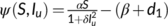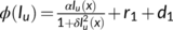Here describes the infection force of the disease and measures the inhibition effect from the behavioral change of the susceptible individuals when the number of infectious individuals increases. Some susceptible class individuals move to the reserved area, which is considered a safe zone during the pandemic. The known infected individuals entered the recovered class after recovered from the COVID-19. Here in this model, we consider the recovered class and the reserved class as the same and denote the density at time by . The model of the study has been taken in the following form

(1)

The above model is defined on the set subject to initial conditions

(2)

where and are the densities at the time of susceptible population, unknown infected population (incubate the illness but do not have any symptoms and not identified), known infected population (in the isolated ward), and recovered or reserved population, respectively, and the parameters , , , , and are all positive. Here, is defined as the total number of population under risk at the time (Figure 1).

The biological meanings of the model parameters are listed below:

The recruitment rate at which new individuals enter the Indian population.

The homogeneous transmission coefficient from the susceptible population () to the unknown infected population (). The rate of transmission of infection is given by .

The parameter measures the psychological or inhibitory effect.

The transmission coefficient from the unknown infected population () to the known infected population (treatment population) ().

The transmission coefficient from the susceptible population () to the recovered or reserved population ().

The transmission coefficient from the known infected population (treatment population) () to the recovered population or reserved population ().

The natural death rate.

The death rate of the known infected class ().

3 ANALYSIS OF THE MODEL AND BASIC PROPERTIES

3.1 Non-negativity of solutions

Theorem 1.Every solution of the system (1) with initial conditions (2) are non-negative for every t 0.

Proof.The right hand side of the dynamical system (1) is completely continuous and locally Lipschitzian on and hence the solution of the system (1) with the initial conditions (2) exists and is unique on the interval with . From the first equation of the system (1) with initial condition , we get

and hence

where

Integrating the second equation of the system (1) with initial condition , the solution can be written in the form as

where

From the third and fourth equations of the system (1) with initial conditions and , we have

and hence

and

and hence

. This completes the proof of the theorem.■

3.2 Boundedness of the system and invariant region

Theorem 2.All solutions of system (1) which lies in are uniformly bounded and are confined to the invariant region defined by as t , where

Proof.Let us assume that is a solution of (1). Since,

(3)

The time derivative of Equation (3) is

For each a , we get

Assuming , we get

Applying the theory of differential inequality (Birkhoff & Rota, 1989), we find that

which yields as . Thus, all solutions of the COVID-19 system (1) which initiate in are uniformly bounded and confined to the region , where . Hence the feasible region with initial conditions (2) is positively invariant region under the flow induced by the system (1) in .■

Remark.All solutions of system (1) have non-negative components, given non-negative initial values in and stay in for t 0 and globally attracting in with respect to the system (1). Therefore, we restrict our attention to the dynamics of the system (1) in . Thus the system (1) with initial conditions (2) defined on is well-posed mathematically and epidemiologically and it is sufficient to study the dynamics of the dynamical system (1) with initial conditions (2) defined on .

3.3 Equilibrium of system

To evaluate the equilibrium points of the system (1), we have to study the zero growth isoclines and the point of interaction. The possible steady-state boundary equilibrium point is , where and . Since the last equation of system (1) does not depend on other equations, we simply study the reduced system

(4)

where is increasing when is small and decreasing when is large. The DFE point becomes , where , and , where . The endemic equilibrium point of the system (4) is , where , , and . The endemic equilibrium point exists if .

4 DFE AND STABILITY ANALYSIS

To eradicate the disease from a varying size population, the more stringent way requires that the total number of the virus-infected population , while a weaker requirement is that proportion sum of the same tends to zero (Busenberg et al., 1991). Thus we need to find the conditions for the existence and stability of the DFE and the endemic equilibrium . Therefore, is the DFE of (4), which exists for all positive parameters.

4.1 The basic reproduction number

The BRN is the average number of secondary infections generated by a single infection and is one of the most vital threshold quantities which mathematically represent the spreading of the virus infection.

The Jacobian matrix of system (4) at an arbitrary point becomes

(5)

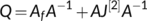
The stability of is equivalent to all the eigenvalues of the characteristic equation of at being with negative real parts, which can be assured by the BRN () obtained by the next-generation matrix method (Van den Driessche & Watmough, 2002), where is the epidemiological threshold parameter.

Let . Then the system (1) can be written as

The Jacobian matrices of and at the DFE are given by

from the above two matrices we get the matrices and as below

The next generation matrix for the system (1) is .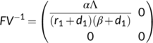

The spectral radius of the matrix is which is the BRN 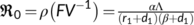. Now, it has been observed that 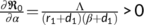. From this observation, it is obvious that if the transmission coefficient from the susceptible population () to unknown infected population () decreases, then the BRN also decreases and therefore reduces the burden on the infection. Otherwise, if increase, then would also increase, and thus, the transmission of virus infection will also rise; therefore, the scenario will be very harmful to society.

Now, the BRN has been presented graphically in Figure 2 with respect to related estimated or hypothetical parameter values given in Table 1. From Figure 2, it is observed that as the value of increases, also increases simultaneously and become greater than unity after a certain value of . Therefore, it is said that up to a certain value of , the DFE point is stable (Theorem 3) and beyond that value of , the endemic equilibrium point is stable (Theorem 6).

TABLE 1. Parameters with their real field value

Parameters	Value	Reference
		Estimated
		Estimated
		Assumed
		Estimated
		Assumed
		Estimated
		Estimated
		Estimated

4.2 Local stability of the DFE

This section will discuss the parameter restrictions of the local stability of DFE.

Theorem 3.The disease free equilibrium of the system (4) is locally asymptotically stable if . Whereas, it is unstable if .

Proof.The variational matrix of the system (4) at is given by

(6)

The eigen values of the characteristic equation of are

For stability, all eigen values must be negative. So, gives

Hence, the DFE is locally asymptotically stable if .■

4.3 Global stability of the DFE

In this section, we will discuss the parameter restrictions of the global stability of DFE.

Theorem 4.When , the disease free equilibrium is globally asymptotically stable in .

Proof.To prove the global stability of DFE when , we choose a suitable Lyapunov function 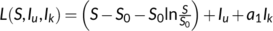. Differentiating along (4), we obtain that

We observe that = 0 if and only if . Therefore, the maximum invariant set in is the singleton set , when . By using Lasalle's invariance principle (LaSalle, 1976), the DFE is globally asymptotically stable in , when .■

5 DISEASE PERSISTENCE

5.1 Uniformly persistence

In this subsection, an effort is made to understand the uniform persistence of the dynamical system (4) for the threshold parameter by applying the acyclicity theorem (Sun & Hsieh, 2010).

Definition 1.The system (4) is said to be uniformly persistent (Butler et al., 1986) if there exists a constant such that all solutions with positive initial satisfy the following inequality

(7)

Let be a locally compact metric space with metric , and let is a closed non-empty subset of with the boundary and interior . Clearly, is a closed subset of and let be a dynamical system on . Then set in is said to be invariant if .

Theorem 5.Suppose the conditions and holds true for the dynamical system

H1:.The system has a global attractor.

H2:.If , then there exists a set

of disjoint, compact and isolated invariant sets in such that

1. There are no subsets of M which form a cycle on ;
2. , where is the omega limit set of
3. Every set is isolated in , 1 i
4. for , where is a stable manifold of .

Then the dynamical system is uniformly persistent with respect to .

Proof.For the modified COVID-19 system (4), we assume that

= : , and . Clearly, . On , the system (4) reduces to , in which as . So it is concluded that and for all which proves (i) and (ii) of . From Theorem 3 the DFE is unstable When and also which indicates that (iii) and (iv) of are satisfied. Since all system (4) solutions are uniformly bounded, a global attractor exists and hence holds true for the system (4). Hence the system (4) is uniformly persistent with respect to , when .■

6 ENDEMIC EQUILIBRIUM AND STABILITY ANALYSIS

From Theorem 4, it is already observed that DFE is globally asymptotically stable when which implies that there is no endemic equilibrium when . To analyze the existence of nontrivial interior equilibrium of system (4), it should satisfy the following conditions:

(8)

with and the above Equations (9) leads to the following solutions as , , and . Clearly but and 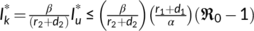are positive if . Hence the nontrivial interior equilibrium of system (4) exists if .

6.1 Local stability analysis of the endemic equilibrium

Theorem 6.The endemic equilibrium of the system (4) is locally asymptotically stable in if .

Proof.The variational matrix of the system (4) at is

where

The characteristic equation of is

(9)

where and . One of the eigenvalues of from the Equation (10) is which is negative. The Routh–Hurwitz conditions state that the quadratic equation has negative roots or complex conjugates with negative real part if and only if and . But after simplification, we get

Obviously for . Hence, the positive equilibrium point is locally asymptotically stable if .■

6.2 Global stability analysis of the endemic equilibrium

To investigate the globally stability of the endemic equilibrium of system (4) when , we apply here a geometric approach (Li & Muldowney, 1996). We begin the preliminary discussion on the geometric approach by formulating the local version of the closing lemma of Pugh (Hirsch, 1991). Consider the differential equation

(10)

where , open set, simply connected and .

Let be an matrix valued function which is in and , where is the matrix obtained by replacing each entry in by its directional derivative in the direction of . Let be the second additive compound matrix of and be the Lozinskii measure (Coppel, 1965) with respect to a vector norm on defined as , I is the unit matrix.

The following quantity is well defined. If there exists a compact absorbing set and the system (11) has a unique equilibrium in , then the unique equilibrium of (11) is globally asymptotically stable in if .

Theorem 7.Assume that . Then there exist such that the unique endemic equilibrium is globally asymptotically stable in the interior of when .

Proof.To prove this result, we find the second additive compound matrix from the Jacobian matrix of (5) for the reduced system (4) at in the following form:

(11)

where

and the matrix function is defined by with . Then . Therefore, the matrix can be written in the following block form as

where , , and

The vector norm of the vector in can be defined as . Suppose be the Lozinskii measure with the above defined norm, so as described in (Martin, 1974) and it follows the condition as , where , , , and are the matrix norm with respect to the vector norm. If denotes the Lozinskii measure with respect to norm. Using the second equation of system (4), we have

Using the third equation of system (4), we have

Since system (4) is uniformly persistent when , there exist and such that implies , , and for all . If , where , then . Therefore, we get . Hence,

which implies that . Thus, the endemic equilibrium of the reduced system (4) is globally asymptotically stable, when .■

7 DISCUSSION AND SIMULATIONS

In this section, firstly we consider the case when the BRN 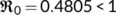by utilizing the parameter values as in Table 1. For different initial conditions, the dynamics of the system (4) is represented in Figure 3. These figures illustrate that the susceptible population () persists and tends to as and the unknown infected population () and the known infected population () tends to zero as , that is, the system (4) approaches the DFE . This numerical simulation supports the result stated in Theorem 4. Next, we consider the case when by utilizing the values of parameter from Table 1 with . For various initial conditions, the dynamics of the system (4) is represented in Figure 4. These figures illustrate that the susceptible population (), the unknown infected population () and the known infected population () all persist, that is, the system (4) tends to endemic equilibrium .

To determine the outbreak of infected individuals of COVID-19 disease in the Indian population, we present the numerical simulation of the proposed dynamical system (1), using MATLAB for simulation experiments, based on the SARS-CoV-2 virus-infected cases in the time frame in India. Here, we employ the nonlinear least-squares curve fitting method with the help of “fminsearch” function from the MATLAB Optimization Toolbox to obtain the best-fit parameters for INDIA. The procedure looks for the set of initial guesses and pre-estimated parameters for the model whose solutions best fit or pass through all the data points by reducing the sum of the square difference between the observed data and the model solution, that is, If a theoretical model is attained and depend on a few unknown parameters and a sequence of actual data points is also at hand then the aim is to obtain values of the parameters so that the error calculated can attain a minimum, where .

For simulation, we assume the initial values are , , from March 25 to April 14, 2020 and , , from April 15 to April 20, 2020.

Figures 5-8 are drawn based on the parameter values (shown in Table 1). The values of the parameters are fixed based on the following real-time data of India, as shown in Table 2, the spread of the COVID-19 disease during the lockdown period is recorded as follows (MoHFW, 2021)

TABLE 2. COVID-19 active cases in India from 25th March to 20th April, 2020

Date
Active cases
Date
Active cases
Date
Active cases

Figure 5 has been drawn for the unknown infected population () and known infected population () for , and for the specified period from March 25 to April 14, 2020 during the first lockdown. This figure is fascinating because it is observed that for , the known infected population curve of our proposed system fits to the curve of the real confirmed infected individuals in India during the above said period.

Figure 6 shows the time history of the unknown infected population () and known infected population () for , and for the period from April 15 to April 20, 2020 during the second lockdown situation. Figure 10 is very interesting because it is observed that for , the known infected population curve of our proposed COVID-19 system fits to the curve of the real confirmed infected individuals in India during the above said period.

Figure 7 shows that the time history of the unknown infected () and known infected () populations of the proposed system corresponding to and fits to the curve of the real confirmed infected individuals in India during the lockdown period from March 25 to April 20, 2020.

It is also clear that as a representative of lack of following the good practices such as proper hand wash, sanitizing the places, nasal, and oral covering with a mask, social distancing has an effect in the proposed coronavirus model and an increase in means many individuals are not following the good practices as said above and as a result, many individuals gets infected and move to the unknown infected population (). Long run prediction of the time history of the known infected population () for and is drawn in Figure 8, which shows that the disease gets diminished may be due to the availability of a Vaccine.

From Figure 8, it is observed that the active cases will decrease and the COVID-19 disease will persist in the society for a long period. Furthermore, it is noticed that the COVID-19 disease diminishes after a long period if people do not strictly follow the government guidelines and vaccination is not found at the earliest as we have considered that geographical and climatic factors do not have any impact on this virus infection.

From Figure 9, it is noticed that if increases, which is a representative of the identification process of the infected individuals, then the unknown infected population reduces and hence we can identify the individuals for quarantine. Thus, the lockdown period can be reduced and people can come back to a normal situation.

Figure 10 shows that if the recovery rate increases, which representing the quality of treatment and cooperation of the patient to the treatment, then the known infected population () tends to zero in the long run. Hence, the rapid spread of COVID-19 disease is reduced drastically.

Figure 11 represents the graphical representation of the day-wise increase of infected, recovered, and deceased population from March 1 to March 20, 2020 in India (COVID19 tracker, 2021). It is observed that active infected cases start to increase from the third week of March because many have already been infected, failed to be in isolation, not strictly adhering to the rules imposed by the Government and ICMR at the time of the second week of March, and hence the active cases increases but in control during the first lock downstage. It is also observed that the day-wise recovered cases are also increasing and day-wise deceased cases are very low. From the above discussions, it can be said that SARS-COV-2 is threatening to the society, but not deadly dangerous until now in Indian perspective.

8 CONCLUSION

The proposed model has determined the outbreak of COVID-19 disease in the Indian population. The BRN is the threshold limit that determines the dynamical proliferation. The reproduction number decreases if the transmission coefficient decreases. If increases, then the transmission of COVID-19 disease increases and is very harmful to society. The system has a unique DFE , which is globally stable if which symbolizes that the disease diminishes eventually. When , the system is uniformly persistent under some conditions, a unique endemic equilibrium is globally stable. The study shows that the infected population who incubate the illness of our proposed system fits well to the real confirmed infected individuals in India during the lockdown period.

By observing the time graph of the known infected class () for various values of , we conclude that if people do not strictly follow the guidelines and lockdown measures imposed by the Government of India to prevent the rapid spread of the infection, the situation will be out of control.

CONFLICT OF INTEREST

The authors declare no conflicts of interest.

AUTHOR CONTRIBUTIONS

Analysis and draft the paper: R. Prem Kumar and Sanjoy Basu. Collected the data, conceived and designed the analysis, perform the analysis tool for the paper: D. Ghosh and P. K. Santra. Supervised, designed the analysis and wrote the paper: G. S. Mahapatra.

CONSENT TO PARTICIPATE

This article does not contain any studies involving animals or human participants performed by any authors. Anyone can read material published in the Journal.

CONSENT FOR PUBLICATION

We, the undersigned, give our consent for the publication of identifiable details, which can include figures and details within the text (“Material”) to be published in the above Journal and Article. Therefore, anyone can read material published in the Journal.