

Imaging of groundwater contamination using 3D joint inversion of electrical resistivity tomography and radio magnetotelluric data: A case study from Northern India
ABSTRACT
The impact of untreated sewage irrigation and waste disposal practices on groundwater is investigated by 3D joint inversion of radio magnetotelluric and electrical resistivity tomography data. In this case study, electrical resistivity tomography and radio magnetotelluric field measurements were carried out on several profiles near a waste disposal site which was irrigated with untreated sewage water for agriculture purpose. In addition, radio magnetotelluric and electrical resistivity tomography measurements were carried out, far away from the waste site, to derive the uncontaminated geology. The data were analysed earlier using 2D inversion techniques. However, for the 2D inversion of the electrical resistivity tomography and radio magnetotelluric data, assumptions about the strike direction are required. As no clear strike direction is evident for the contamination, we considered the problem as 3D and interpreted the present data set using the 3D inversion algorithm ‘AP3DMT-DC’. The inverted 3D resistivity model shows an unconfined aquifer of low resistivity which is overlain by an unsaturated slightly resistive near surface formation. With increasing distance from the waste sites, an increase in the resistivity of the shallow unconfined aquifer is observed. Furthest away from the waste site undisturbed geology is expected. We derived consistent and meaningful 3D resistivity models. The uncontaminated reference site indicates an increased resistivity for the aquifer layer. A synthetic 3D study was carried out to demonstrate and validate algorithm performance as well as convergence capabilities. The study demonstrates that the two methods, electrical resistivity tomography and radio magnetotelluric, complement each other. Besides, a better resolved inverted model is obtained through a 3D joint inversion, in comparison to individual 2D and 3D inversions.
INTRODUCTION
The electrical resistivity tomography (ERT) and radio magnetotelluric (RMT) methods are commonly used for shallow subsurface investigations (Linde et al. 2004; Diaferia et al. 2008; Bastani et al. 2012; Carpenter, Ding and Cheng 2012; Yogeshwar et al. 2012; Pidlisecky et al. 2016; Devi et al. 2017; Dahlin and Loke 2018; Ikard and Pease 2018; Kiseleva et al. 2018;Walter et al. 2019). ERT is an active method, where the current is injected directly into the ground and the potential difference is measured on the surface of the earth. The RMT method utilizes remote radio transmitters as source fields in the frequency range from 10 kHz to 1 MHz. Transfer functions are derived from two orthogonal electric and magnetic field components, measured on the earth's surface. The plane electromagnetic source signals induce secondary electromagnetic fields from which apparent resistivity and phase values can be derived (Linde and Pedersen 2004; Tezkan, Hördt and Gobashy 2000, 2008; Tezkan, Muttaqien and Saraev 2018).
Since the sensitivity of ERT and RMT methods is different for resistive and conductive structures, inversion of ERT and RMT data can be performed either (i) separately, where the two resulting models are integrated and interpreted (e.g. Diaferia et al. 2008; Seher and Tezkan 2007; Shan et al. 2014) or (ii) jointly, where the two different data sets are judiciously merged into one data set to constrain the interpretation (Tezkan et al. 1996; Candansayar and Tezkan 2008; Bastani et al. 2012). In view of the fact that the potential limitation of one method can be compensated by the strength of the other, we performed a 3D joint inversion.
The ERT and RMT methods are widely used to study hydrogeophysical problems, such as groundwater contamination, aquifer delineation, sewage leakage and detection of leakage pathways in earth-filled dams (Pedersen, Bastani and Dynesius 2005; Sudha et al. 2010; Yogeshwar et al. 2012; Metwaly et al. 2014; Pidlisecky et al. 2016; Abu Rajab, El-Naqa and Al-Qinna 2018; Moghadas and Badorrech 2019; Perdomo, Kruse and Ainchil 2018; Høyer et al. 2019; Plank and Polgar 2019; Sarntima, Arjwech and Everett 2019).
In the present work, we analysed ERT and RMT data sets acquired around the waste disposal and untreated sewage water irrigation site in Saliyar village, located near Roorkee in Northern India. The study took place within Indo-German scientific cooperation. 2D joint inversion of this data set was presented by Yogeshwar et al. (2012). Sudha et al. (2010) carried out RMT and time domain electromagnetic (TEM) soundings in the same area. Von Papen, Tezkan and Israil (2013) performed quasi 3D inversion of TEM data to study the effect of groundwater contamination. These earlier studies identified increasing subsurface resistivity as moving away from the waste site, which can be a source of groundwater contamination due to untreated sewage water irrigation. In this study, we performed 3D joint inversion of ERT and RMT data. Initially, we discussed the survey area and the inversion methodology. Afterwards, we investigated the capabilities of the algorithm ‘AP3DMT-DC’ (Singh 2018) for the 3D ERT and RMT joint inversion on the basis of a synthetic model. Subsequently, we presented the 3D inversion of ERT and RMT field data for both single and joint data sets.
The aim of this work is (i) to derive a 3D model that can explain ERT and RMT data simultaneously, (ii) to investigate the benefits of jointly inverting both data in order to improve the subsurface resolution and (iii) to provide an improved and more realistic 3D subsurface resistivity model of the Saliyar sewage site, which is used for the assessment of groundwater contamination potential.
SITE DESCRIPTION AND FIELD SURVEY
The study area is situated around the waste disposal site in Saliyar village located between 29°53'N to 29°54'N and 77°51'E to 77°52'E (Fig. 1). The area lies in the lower piedmont zone, also known as the Tarai zone, of the Himalayan foothill region, around Roorkee, Uttarakhand, India. The area comprises mostly unconsolidated alluvial sediments of the Quaternary period. The sediments of the area consist of alternating layers of clay, sand, pebble and gravel in some places. The general lithology comprising the top soil layer of thickness 3–6 m is sandy loam, with approximately equal distribution of soil, sand, silt and clay (Singhal et al. 2003). Below this lies the shallow unconfined aquifer of 3–27 m thickness, which, in turn, is underlain by a second aquifer of about 14 m thickness. The two aquifers are separated by a clayey layer intermixed with gravel.

The southeasterly flowing Solani River is located at a distance of approximately 500 m from the waste disposal site in the northwest direction (Fig. 1). In the southeast direction, groundwater flow is controlled by gentle elevation and slope and is almost parallel to the Solani River (Singhal et al. 2003; Bhatnagar, Joshi and Singhal 2004).
Many researchers have studied the contamination in groundwater, due to waste disposal and untreated sewage irrigation practices in the region, using the physiochemical parameters of groundwater (Singhal et al. 2003; Bhatnagar et al. 2004; Kamboj et al. 2015). All of them found that the upper aquifer near the Saliyar village is contaminated due to the sewage water irrigation. Bhatnagar et al. (2004) investigated that the heavy metal (viz. Cd, Co, Cu, Fe, Pb, Mn, Ni and Zn) concentration is high in the plots irrigated with untreated sewage water, and moderate to severe water contamination is observed in some parts. Singhal et al. (2003) indicated that the value of total dissolved solids is high in groundwater of the upper unconfined aquifer of Saliyar village. Electrical resistivity tomography (ERT) and radio magnetotelluric (RMT) data were acquired in this region to image the different zones of contamination.
Yogeshwar et al. (2012) recorded in total 8 ERT and 13 RMT profiles, using the ABEM Terrameter SAS 1000 and the RMT-F device, from the University of Cologne (Tezkan and Saraev 2007; Tezkan 2009), respectively. Of these, we are inverting only the 6 ERT and 10 RMT profiles that are located between the waste disposal site and the Solani River (Fig. 1). It should be mentioned that profile ‘R03’, on the right bank of the Solani River, is far away from the waste disposal site and is treated as a reference profile corresponding to the uncontaminated zone. The profiles, as shown in Fig. 1, are mainly oriented in the southeast direction and are parallel to each other except for the profile PR13, which is perpendicularly oriented. The profiles are labelled PR01 to PR13 as shown in Fig. 1. The distance between two consecutive profiles is roughly 50 m. The total area being covered is approximately 200 × 650 m2. The area above the waste disposal site was not accessible for measurements.
Wenner and Schlumberger, short and long, configurations were used for ERT data acquisition, with a profile length of 200 m (excluding profile PR03, which is 120 m long). The inter-electrode spacing of 5 m and 2.5 m was used for the outer and middle parts of the profile, respectively.
The RMT profile length is 200 m; for most of the profiles, the inter-station spacing is 10 m. For profiles PR01 and PR03, the length is approximately 100 m. Five to six frequencies, in the range 10 kHz to 1 MHz, were used for both E-polarization (TE-mode, i.e. transmitters associated with the electric field directions are in line to the presumed strike) and B-polarization (TM mode, i.e. transmitters are perpendicular to presumed strike). The E-field parallel to the profile line was therefore assumed as TM mode for the 2D inversion of the RMT data. The acquisition parameters of RMT data are shown in Table 1.
| Profile name | Number of stations | Profile length |
|---|---|---|
| PR01 | 9 | 80 |
| PR02 | 21 | 200 |
| PR03 | 10 | 100 |
| PR04 | 18 | 170 |
| PR05 | 18 | 170 |
| PR06 | 20 | 190 |
| PR07 | 20 | 190 |
| PR08 | 19 | 180 |
| PR13 | 21 | 200 |
| R03 | 21 | 200 |
The distribution of groundwater contamination is, in many cases, 3D; therefore, a definite strike direction cannot be identified. If no clear strike direction is identified, the subsurface distribution of contaminants due to untreated sewage needs to be considered as 3D. Consequently, a 3D interpretation of the acquired ERT and RMT is beneficial, although our survey design was oriented along profiles. The 3D model will help not only in the estimation of groundwater contamination but also in finding the general flow direction of groundwater/contamination.
INVERSION METHODOLOGY
 (1)
(1)For the convergence and accuracy of the iterative procedure, optimal values of few inversion parameters are required: (i) regularization parameter, (ii) iteration and tolerance for BiCGSTAB, (iii) data weighting matrix, (iv) 3D forward and inverse modelling grid parameterization and (v) starting model resistivity.
The initial value of the regularization parameter (λ) is chosen to be 10 on the basis of an L-curve analysis (Hansen and O'Leary 1993; Meqbel 2009). The tolerance parameter of BiCGSTAB is chosen to be 10−10. The finite-difference grid is denser near the electrodes, where potential gradients are large and the grid is progressively coarser towards the external boundaries, and the boundary conditions have to be satisfied (Fig. 2). For the vertical direction, the first grid spacing below the surface is fixed at approximately one-fourth of the minimum electrode spacing, and subsequent spacings are increased by a constant factor (1.2). Average apparent resistivity of ERT data was used as the initial guess model for all ERT and RMT individual and joint inversions.

 (2)
(2) for the data set 2 is computed by using the norm of both gradients:
 (3)
(3) are the data misfits for each ERT and RMT data set, respectively. This joint inversion scheme incorporates both (i) the weighting with the number of data points and (ii) the resolution capacity of each method because the sensitivity is reflected in the gradient calculation.
Another important criterion for choosing the weighting factors is the error estimates in each data set such as the total number of data points (Candansayar and Tezkan 2008) or depth of investigation (DOI)-based weighting (Sudha et al. 2010). If the errors in the data covariance matrix are overestimated and therefore too large, it will result in a large non-uniqueness and a poorly resolved model. In contrast, if the errors are underestimated, the inversion may not converge.
 while that of RMT data by unity, the desired nRMSopt is calculated as
 (4)
(4)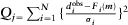 . Here, j refers to either ERT or RMT misfit. Nd = NRMT + NERT is the total number of data, NRMT and NERT are the number of RMT and ERT data points. N is the total number of data points for respective method;
  is the ith observed data;
  is the ith synthetic data and
  is the data standard error in ith observed data value. An nRMS = 1 indicates optimal data fit with respect to the error bars. After re-weighting, the error bars in data values change, and the desired nRMS gets modified automatically.
RESULTS
We initiated the 3D inversion by first performing a synthetic experiment on a canonical model. The synthetic experiment helps us in defining the inversion parameters for field data inversion and validation of the algorithm.
3D synthetic data inversion
To validate our 3D inversion algorithm using a synthetic model, we computed the electrical resistivity tomography (ERT) and radio magnetotelluric (RMT) model responses using the Res3DMod (Loke 2013) and ModEM (Kelbert et al. 2014) algorithms, respectively.
The synthetic model consisted of two blocks having resistivity values of 10 Ωm and 1000 Ωm, respectively (Fig. 3), and a background half-space of resistivity 100 Ωm. Such types of 3D models are widely used to demonstrate the code performance and convergence capabilities (e.g. Boonchaisuk, Vachiratienchai and Siripunvaraporn 2008; Grayver 2015; Kruglyakov and Kuvshinov 2019). Each block had a dimension 60 × 30 × 15 m. These blocks were placed at a distance of 20 m from each other in the y-direction. The top of two blocks was 5.4 m below the surface. The model was discretized into 36 × 36 × 20 cells with horizontal cell dimensions of 5 m. For vertical discretization, the first grid mesh size was at a distance of 1 m below the surface. The thickness of each subsequent layer was increased by a factor of 1.2, extending down to 1 km. A total of 24 cells were padded around the central region, six in each horizontal direction with increasing width. With this mesh, the dimension of the model domain becomes 2 × 2 × 1 km in the x-, y- and z-directions, respectively. The true model, in the form of depth slices, is shown in the first column of Fig. 3. A homogeneous model of 100 Ωm was used as an initial model for the 3D inversion.

We used Schlumberger configuration with an inter-electrode spacing of 5 m to generate synthetic ERT data. The spacing between each profile was 10 m. To simulate realistic field conditions, 5% Gaussian noise was added to the responses. Accordingly, the error bars were set to 5% of the absolute response values. The algorithm converges from 9.90 to a final optimal nRMS of 1.03 in 26 iterations. The nRMS for individual inversion was calculated according to Eq. 4 considering either ERT or RMT data. The inverted resistivity model in form of depth slices is shown in the second column of Fig. 3.
The RMT off-diagonal apparent resistivity and phase responses were generated for 12 logarithmically equidistant frequencies in the range from 10 kHz to 1 MHz. The stations were located on 11 profiles with 11 stations on each profile and an inter-station spacing of 10 m (Fig. 3). The station numbering starts with 1 from x = −52 m, y = −47 m and are numbered along the y-direction. A 5% Gaussian noise was added to the computed response. The data errors were set to 5% of apparent resistivity and phase for both off-diagonal apparent resistivity and phase. Convergence was reached after 46 iterations, while the nRMS value reduced from 9.84 to ∼1.10. The inverted resistivity model in the form of depth slices is shown in the third column of Fig. 3.
Lastly, the joint inversion of the ERT and RMT data sets was performed using the same data and model parameters as in the single inversion cases. Since the norm of the gradient of the RMT data was larger, additional up-weighting was done for ERT data by a factor of 3.40 (Eq. 3). The new target nRMS value was found to be 1.16 (Eq. 4). In the 3D joint inversion, the nRMS reduced from 15.73 to 1.68 in 56 iterations. The inverted model in the form of depth slices is shown in the fourth column of Fig. 3 while Fig. 4 displays the data and fitting for off-diagonal components of apparent resistivity (Rho) and phase (Ph) for selected RMT stations. The data are well fitted throughout the complete period range. The misfit is displayed as a colour-coded ERT pseudo-section, in Fig. 5, for one profile located at x = −2.50 m.


The 3D inversion of synthetic data is meaningful and consistent with respect to the resolution capabilities of each single method. RMT as an induction method shows better resolution for the resistivity value of the conductive block, whereas ERT reconstructs the resistive block slightly better. The overall resistivity values are depicted best when inverting both methods jointly. Both blocks are slightly smeared out at depth due to the lack of resolution and the imposed vertical smoothness constraints. At shallow depth between 7.4 m to 12.9 m, the block geometry appears to be slightly better reproduced by the RMT individual inversion. This is also reflected in the joint inversion results. At 20.8 m (i.e. bottom of the blocks) both methods lack geometrical resolution. Overall, the synthetic study demonstrates the applicability to reconstruct 3D geometries and performance of the algorithm.
3D field data inversion
The ERT and RMT data acquired at the waste site were inverted individually and jointly for the contaminated area and for an uncontaminated reference profile labelled as R03. The resistivity models of the individual 2D inversion for ERT and RMT data of the reference profile, R03, carried out by Yogeshwar et al. (2012) are shown in Fig. 6(a,b), respectively. For comparison, a 3D inversion was performed individually, the ERT (Wenner array) and RMT (off-diagonal apparent resistivity and phase), and jointly for the reference profile R03. The obtained resistivity models are shown in Fig. 6(c–e) for profile location at x = 600 m. Our results compare well to those obtained by Yogeshwar et al. (2012), and all relevant features are reconstructed. It should be noted that it is rather unusual to perform 3D inversion of a single profile. However, 3D inversion of profile data is useful to account off-profile structure. 3D inversion of profile data can account off-profile resistivity structure in right place and improve data fit (e.g. Newman et al. 2003; Siripunvaraporn, Egbert and Uyeshima 2005; Ivanov and Pushkarev 2012; Devi et al. 2019). However, off-profile structure may the distort final inverted resistivity model in 2D inversion.

Figure 7(a–c) displays the results as slice view for the 3D individual and joint inversion of all ERT and RMT profiles. The data along the 5 ERT profiles (PR02-PR08) displayed in Figs 1 and 2 were used for the 3D inversion. The dimension of the 3D modelling domain is 2755 m × 2880 m × 400 m in the x-, y- and z-directions, respectively. To ensure accuracy and spatial resolution, additional 24 cells were included in the central part of the model, six in each horizontal direction, with the distance increasing by a factor of two (cf. Fig. 2). According to electrode spacing, the mesh size used in the central part of the model was 2.5 m for the x-direction (i.e. profile direction). For the y-direction (i.e. perpendicular to the profiles), the mesh size was adjusted to 7.5 m around the profiles and even 15.0 m wide in the middle of two consecutive profiles. A horizontal view of the grid is depicted in Fig. 2. The minimum mesh size was 1 m (first) in the vertical direction and increases by a factor of 1.15 with depth. A homogeneous half-space model with 34 Ωm resistivity was used as a starting model according to the calculated average of the observed ERT apparent resistivity values. The total number of ERT Wenner and RMT data points was NERT = 1413 and NRMT = 2823, respectively. All acquisition and inversion parameters for the single and individual inversion runs are given in Table 2. The inverted resistivity model for the ERT Wenner array configuration is shown in Fig. 7(a).
| Error floor (%) | |||||
|---|---|---|---|---|---|
| Data type | Apparent resistivity | Phase | Starting nRMS | Final nRMS | No. of iterations |
| ERT (R03 profile) | 5 | – | 4.67 | 1.45 | 55 |
| RMT (R03 profile) | 5 | 2.5 | 18.60 | 2.26 | 69 |
| ERT + RMT (R03 profile) | 5 | 2.5 | 21.20 | 2.49 | 103 |
| ERT (5 profiles) Wenner array | 5 | – | 14.67 | 1.89 | 64 |
| RMT (9 profiles) | 5 | 2.5 | 35.73 | 3.03 | 59 |
| ERT + RMT (5 + 9 profiles) | 5 | 2.5 | 20.05 | 2.46 | 109 |

In the case of RMT data, 3D inversion of nine RMT profiles with an inter-station spacing of 10 m and an inter-profile spacing of 35 m was performed. The RMT off-diagonal components of apparent resistivity and phase in the frequency range from ∼1 kHz to ∼1 MHz were used as input. The number of frequencies varies at each station due to limited availability of transmitter signals during recording. However, usually 5 to 6 stable frequencies were available at each station. The inverted 3D RMT model is shown in Fig. 7(b).
Subsequently, ERT and RMT data were then jointly inverted using all N = 4236 data points. The norm of the RMT gradient of the misfit functional was larger. Therefore, an up-weighting by a factor of 1.63 was done for ERT data. Accordingly, the inversion converges to an nRMS value of 2.46 in 109 iterations. To maintain consistency, the inversion control parameters, model dimension and discretization were kept the same as in case of the individual data inversions. The inverted 3D model in the form of resistivity-depth sections is shown in Fig. 7(c). The derived 3D models are in good agreement and provide a spatially consistent structure. Higher resistivities are in general observed towards the southern zone and along profile R03. The joint inversion result also reveals a more resistive layer occurring at a depth of roughly 10 m below conductive layering. The latter is not observed in the individual inversion.
Figure 8 displays the data and fitting of the apparent resistivity and phase for nine selected soundings along each one exemplary RMT profile. The data are well fitted for both apparent resistivity and phase. In Fig. 9, the data misfit is plotted for the exemplary ERT profile PR05, in the form of a colour-coded percentage relative difference pseudo-section. The pseudo-section shows that the misfit is mainly less than 2% except for few outliers.


Sensitivity test
 (5)
(5)where ρ is the resistivity and f is the frequency and the DOI in m is estimated approximately to 21.3 m. We assume an 8 Ωm half-space and a minimum frequency of 10 kHz. To further validate the resistive feature, we performed a sensitivity test by replacing the resistive feature with a 10 Ωm conductive feature. Subsequently, we computed the corresponding forward response and calculated the data fit. The nRMS error value significantly deteriorated from 2.46 to 4.22. Thus, the significant increase in nRMS error value and DOI of 21.3 m indicates that the resistive feature in joint inversion is not an inversion artefact but is an essential feature.
DISCUSSION
Geologically, the study area consists of alluvial sediments, of recent age, deposited by the Himalayan rivers. The Solani River, flowing in the southeast direction, influences the local hydrogeology and groundwater flow. On the basis of groundwater table elevation contour maps, Singhal et al. (2003) estimated that the groundwater flow in the studied region is also in the southeast direction. The direction of groundwater flow is indicated by an increase in the depth of water table elevation by a red arrowhead line in the resistivity section for profile PR02 in Fig. 7(b).
Reference profile R03
Resistivity-depth sections of the reference profile R03 (Fig. 6) show a low resistivity (15–25 Ωm) zone labelled ‘A’ and a high resistivity (60–200 Ωm) zone labelled ‘B’ for near-surface (< 10 m) formation. These two zones vary to some extent in their geometry and resistivity value in the different sections. The low resistivity zone ‘A’ represents a water-saturated region comprising upper unconfined aquifer layer (Singhal et al. 2003), whereas the resistive feature ‘B’ represents the presence of unsaturated coarser material with gravels. Below the depth of 10 m lies the saturated layer (resistivity 12–40 Ωm) of the unconfined aquifer. This zone is more clearly visible in the inverted model obtained from radio magnetotelluric (RMT) data (cf. Fig. 6d).
Waste site profiles
In Fig. 6(c,d) as well as Fig. 7(a–c), the resistivity models for the reference profile ‘R03’ show a top thin (∼1 m thick) resistive layer corresponding to the dry surface fine sand layer of the Solani River bed. It is underlain by a low resistivity layer, representing the upper unconfined aquifer zone. The 3D resistivity-depth sections (Fig. 7) obtained from data on profiles (PR03–PR07) near the waste disposal site shows low resistivity values right from the surface. These zones were irrigated with sewage when the survey took place. The low resistivity zones indicate the presence of possible contamination in groundwater due to sewage water irrigated agricultural fields. In the depth section of profile PR02, the high resistivity of the near surface zone is a result of an artificial landfill and unsaturated soil. Some localized high resistivity zones are observed along profiles PR03 and PR07. These possibly correspond to large size boulders as often occur in Himalayan foothill regions or dry/unsaturated zones. The low resistivities suggest that the entire unconfined aquifer around the waste site area is affected by the contamination due to untreated sewage water irrigation.
The depth slices extracted at five different depths for 3D models, obtained from the two individual and the joint inversion of electrical resistivity tomography, RMT data, are shown in Fig. 10. The resistivity slices indicate the absence of low resistivity at depths greater than 16 m, which is also shown in Fig. 7(c). The contaminated water is, probably, not reaching beyond a depth of 16 m. It was earlier discussed by Bhatanagar, Joshi and Singhal (2004) that water extracted from deeper wells (z = 18–60 m) is more suitable as compared with the shallow handpump water (z < 18 m). This may be due to the presence of a non-permeable layer below the unconfined aquifer. The lithology in the area suggests that the higher resistivity below the unconfined layer is due to the presence of gravel and coarser material.

CONCLUSION
The electrical resistivity tomography (ERT) and radio magnetotelluric (RMT) data recorded near the waste disposal site in Saliyar village, Roorkee, were interpreted using 3D individual and joint inversion technique. For this purpose, the recently developed 3D joint inversion code ‘AP3DMT-DC’ was used for ERT and RMT data inversion. The code was first validated through a synthetic example. The geometry and resistivity of the subsurface formation are revealed in the inverted model. The iterative scheme converged well in both cases, the individual and joint 3D inversion, at a similar speed. The 3D inverted profile sections are consistent in itself and with the corresponding 2D inversion results. The derived models are meaningful with respect to the general hydrogeological understanding of the area. Moreover, the 3D resistivity profile sections, down to a depth of 16 m, show a low resistivity representing an upper unconfined aquifer affected by the groundwater contamination. The resistivity increases below a depth of 16 m indicating that the contamination is not reaching deeper depths. The 3D resistivity model obtained by the joint inversion of ERT and RMT data better explains the resistivity variation and geometry of all the features than the models obtained by individual inversions. The 3D model helps not only in the estimation of groundwater contamination but also in finding the general flow direction of groundwater and possible contaminants.
ACKNOWLEDGEMENTS
The data used in this paper were recorded in a joint research project funded by DFG (Deutsche Forschungsgemeinschaft) and DST (Department of Science and Technology, India) and were analysed under a DST-DAAD project. The authors are thankful to all students and research scholars who had participated in the fieldwork. The authors thank Madam Mamta Gupta for language editing. We thank the two reviewers for valuable comments and suggestions that significantly helped to improve the manuscript.

