An analysis of high order FEM and IGA for explicit dynamics: Mass lumping and immersed boundaries
Summary
We investigate the behavior of different shape functions for the discretization of hyperbolic problems. In particular, we consider classical Lagrange polynomials and B-splines. The studies focus on the performance of the these functions as a spatial discretization approach combined with an explicit time marching scheme. In this regard, a major concern is the maximum eigenvalue that imposes restrictions on the critical time step size and suitable lumping techniques that yield a diagonal mass matrix. The accuracy of the discretization methods is assessed in an asymptotic manner in terms of the convergence of eigenvalues and eigenvectors. Further, the global accuracy is investigated in terms of the full spectrum. The results show that B-spline discretization with a consistent mass matrix are more accurate than those based on Lagrange shape functions, which holds true in the boundary-fitted as well as in the immersed setting. On the other hand, Lagrange shape functions are more robust with respect to standard lumping techniques, which cannot be directly applied for B-splines without loss of accuracy. In general, we observe that none of the standard lumping schemes yields optimal results for B-splines, even in the boundary-fitted setting. For the immersed setting, also Lagrange shape functions show a drop in accuracy which depends on the position of the boundary that cuts the element. Several remedies are considered in order to overcome these issues, including interpolatory B-spline bases as well as eigenvalue stabilization methods. While accuracy and stability can be improved using these remedies, we conclude from our study that it is still an open question, how to design a discretization method that achieves large critical time step sizes in combination with a diagonal mass matrix and high accuracy in the immersed setting. We note that these considerations primarily relate to linear structural dynamics applications, such as for example, structural acoustics. In nonlinear problems, such as automotive crash dynamics, other considerations predominate. An example of a one-dimensional elastic-plastic bar impacting a rigid wall is illustrative.
1 DEDICATION
Our paper is dedicated1 to Professor Robert L. Taylor, better known simply as “Bob”. Bob has been a stalwart in the growth of the field of Computational Mechanics from its inception. He ostensibly retired from the University of California at Berkeley in 1994 at the age of 60, but that was an illusion as he has remained active ever since. That year I organized a conference for Bob, in collaboration with good friends Eugenio Oñate and Olek Zienkiewicz, in Palo Alto in honor of his 60th birthday. It was scientifically interesting and great fun, especially the banquet at the Fogarty Winery high in the hills above Palo Alto. The cliff hugging drive to the winery was too much to take for some of the participants but we all arrived there safely and returned alive, after an outstanding dinner prepared by a top visiting chef and his team. At that time, I didn't think we would once again be celebrating Bob's contributions to the field 30 years later, but here we are. The beat goes on, and on, and on.
I first met Bob shortly after arriving in Berkeley in pursuit of my PhD in August 1969. Bob left for his first sabbatical in Swansea in September 1969 and I did not interact with him until the last year of my PhD when we began to work together on contact-impact problems.2 That work broke ground in one of the most important areas of computational analysis, namely, automotive crash analysis, but that was not the limit of our endeavors. Every day we met for coffee in a cafè in the morning and in the afternoon we would compute. We worked on reduced/selective integration methods to alleviate locking in plates and shells and the incompressible behavior of solids and fluids; structural dynamics algorithms; consistent tangents in constitutive integration; the F-bar formulation for nonlinear elasticity; and the precursor to FEAP (the Finite Element Analysis Program), namely MINIFEM. Bob's continued development of FEAP has provided the computational solid and structural analysis communities with an essential research and development platform to this day. For his many contributions to Computational Mechanics, Bob has received many awards and honors. Here are a few: The T.Y. and Margaret Lin Professorship of Engineering at U.C. Berkeley, the Berkeley Citation, election to the National Academy of Engineering, several honorary doctorates, the Von Neumann Medal of the United States Association for Computational Mechanics (USACM), the Gauss-Newton Medal of the International Association for Computational Mechanics (IACM), the Drucker Medal of the American Association of Mechanical Engineers (ASME), and election to Honorary Fellow of IACM. However, these awards to do not fully represent what Bob means to the Computational Research community and to me personally. His greatness has many dimensions starting with being a great researcher, but also a great teacher, a great mentor, a great collaborator, and a great friend. Bob, you are all those things and have been for your entire career. I am so happy to have the opportunity to collaborate with some of our other friends and dedicate this paper to you.
2 INTRODUCTION
Hyperbolic problems are ubiquitous in engineering. Structural dynamics is a prime example and the focus of this study. We are interested in exploring the spatial discretization possibilities within finite element and isogeometric (i.e., spline based, finite element) analysis for this class of problems, and in particular the comparison of consistent versus lumped (i.e., diagonal) mass matrices and the competition between boundary-fitted and immersed discretizations.
Lumped masses, although generally not variationally consistent, are the rule in explicit transient analysis, which is the dominant technology in crash dynamics and other applications with strong nonlinear behavior. The attributes of explicit dynamics are its minimal computer memory requirements, as there are no matrices involved in solution, its speed of solution per time step, and its robustness in the face of the most challenging nonlinear behavior, which includes contact-impact phenomena, very large plastic deformations, and fracture. The industry standard mesh size in full car crash analysis is 2–3 mm and so these problems are very large and tax computer resources, necessitating the minimal memory footprint of explicit dynamics with lumped masses. It is important to understand that in this class of problems accuracy, in the form of convergence rates, is limited by nonlinear behavior, independent of the formal accuracy of the discretization method in linear problems. It is often mentioned that a shortcoming of explicit dynamic analysis is the very small size of critical time steps. While this is true, there are countervailing benefits to small time steps: They are the main reason explicit dynamic analysis is robust with respect to strong and abrupt nonlinear behavior, and they also a priori guarantee negligible time-integration errors.
There are also many other important structural dynamics phenomena that are dominantly linear, for example, structural acoustics. Here the situation is quite different from crash dynamics, and the possibility of higher-order accuracy presents itself. Classical spectral metrics, namely eigenfrequency and eigenvector errors, are relevant, as well as convergence rates of various quantities in integral norms. One of the questions we are interested in addressing is the effect of discretization procedures on the size of critical time steps, and this can be done within the framework of linear analysis, as the critical time step is inversely proportional to the largest frequency of the discrete model. Although boundary-fitted meshes are generally considered the gold standard in analysis, some very interesting and surprising results have been obtained for the effect of immersed methods on critical time steps. We are interested in understanding this phenomenon more fully. In the context of linear structural dynamics attributes, lumped mass methods will often disappoint compared with consistent mass matrices. Nevertheless, in applications such as crash dynamics, they are essential, for the reasons mentioned above.
In linear structural dynamics the lowest frequencies and corresponding modes of vibration (i.e., eigenfunctions), are of prime interest, although intermediate modes are often of importance in, for example, the dynamics of machines. The highest modes in the discrete spectrum are usually significantly in error for any discretization method, and so are ignored or suppressed through the time-stepping method. We employ the standard central difference method in this work. While there exist several studies on improved explicit time marching schemes, see, for example, References 2-4, these are not relevant given our exclusive emphasis on spatial discretization properties.
In summary, the plan of this paper is to evaluate the spatial discretization properties of lumped and consistent mass, boundary-fitted and immersed, structural dynamics methods, from the standpoints of spectral accuracy, convergence rates and critical time step size. Our goal is a method with a high accuracy and a diagonal mass matrix that yields a low largest eigenvalue.
Considering boundary-fitted discretizations, the spectral element method is favorable in this regard. Using Lagrange polynomials based on Gauss-Lobatto-Legendre points and a nodal quadrature, the resulting mass matrix is diagonal by construction. Further, the largest eigenvalue is underestimated and the asymptotic accuracy is higher than that of a classical finite element methods based on an exact quadrature. For studies of the spectral element method, the reader is referred to References 5-9.
Considering fictitious domain methods, where the physical domain is immersed into an extended domain that can be meshed in a simple way, there is much less clarity in the literature about the mentioned desired properties. While References 7, 8 show that lumping schemes can be applied to recover a diagonal mass matrix for elements cut by the immersed boundary a detailed analysis of the resulting impact on the accuracy of the method is not provided. The present study aims at such a detailed analysis, including an investigation of the effect of the position of the cut in the element on the accuracy and the largest eigenvalue. We restrict our study to one-dimensional problems, such that standard lumping techniques (row summing and diagonal scaling or HRZ lumping) are equivalent to the nodal quadrature for uncut elements as shown in Reference 10. Recently, a reduction in the accuracy due to lumped cut elements was observed in Reference 11, where a combination of implicit (in cut elements) and explicit (in uncut elements) time integration scheme commonly known as IMEX schemes is applied.
As it was shown in References 12, 13, badly cut elements that have only little support in the physical domain lead to extremely high largest eigenvalues which approach infinity as the support approaches zero. A similar phenomenon occurs with enriched finite element bases in the context of the extended finite element method (X-FEM). This was investigated previously in References 14 and 15, which both propose a block-diagonal mass matrix that yields a bounded largest eigenvalue. However, we restrict ourselves here to classical methods that yield truly diagonal mass matrices. Nevertheless, methods like the one mentioned above, as well as tailored time integration schemes and element technologies investigated as early as in References 16, 17, and 18, respectively, provide promising remedies to similar problems as those encountered here as a consequence of immersed boundaries. An overview on the development of such methods at that time is provided in References 19-21.
As an alternative to the continuous discretizations resulting from classical finite and spectral element methods, we investigate the suitability of continuous discretizations with B-splines resulting from an isogeometric analysis (IGA). Since its introduction in Reference 22, IGA has grown to one of the most popular discretization methods and a competitive alternative to finite-element methods. In particular, its superior spectral accuracy as demonstrated in References 3, 23 has rendered it a favorable tool for the solution of dynamic problems in the time and in the frequency domain. Due to the higher continuity, the bifurcations or optical branches in the spectrum observed for continuous discretizations are not present. Therefore, a much larger part of the discrete spectrum has good approximation properties.
However, it is well known that B-spline shape functions lose the high convergence order (asymptotic accuracy) for dynamic problems when a lumped mass matrix is used, see, for example, References 23, 24. In References 25, 26 also the effect of lumping on the global accuracy of eigenvalues was investigated and in Reference 27 the accuracy of eigenvectors was addressed. All of these studies are concerned with boundary-fitted discretizations and find that lumping is not directly applicable without a loss of accuracy. Different strategies are proposed to overcome this issue, some of which we will address in more detail in this paper.
On the other hand, recent studies in References 12, 13 have highlighted a profound advantage of B-splines in combination with a lumped mass matrix when considering immersed problems: if the underlying grid, respectively the knot vector, is designed such that the immersed boundary is far away from the grid boundary, respectively the outer knot spans, the largest eigenvalue is bounded.
In summary, Lagrange shape functions suffer from large maximum eigenvalues in the immersed setting and it is not clear, how lumping in cut elements affects their accuracy. B-spline shape functions suffer from a loss of accuracy when a lumped mass matrix is used and it is not clear how the global accuracy of eigenvectors is affected. Further, the global accuracy of eigenvalues and eigenvectors has not yet been studied in the immersed setting.
The present study aims at a detailed analysis of these aspects. As a starting point, we review the findings from the mentioned studies which are often times performed for a particular application scenario and reproduce them using a common one-dimensional benchmark case. We further enhance the investigations mainly in two aspects. Firstly, we consider not only the boundary-fitted case but include in our studies immersed problems resulting from a fictitious domain approach. Secondly, we consider not only the asymptotic spectral accuracy, that is, the convergence of the first modes, but also the global accuracy considering all modes as done in Reference 3 for the boundary-fitted case. Further, we investigate the properties of the different discretization methods for the solution of selected problems in the time domain.
The paper is structured as follows. In Section 3, we introduce the methodology, that is, the considered hyperbolic problem and its discretization using Lagrange polynomials and B-splines. In Section 4, we explain the conducted numerical investigations in the frequency and in the time domain. The results are presented in the sections thereafter, where in Section 5 we only consider results obtained with consistent mass matrices while in Section 6 we consider only those obtained with lumped mass matrices. We include only the classical FEM and IGA in these sections. In Section 7, we review existing strategies to overcome the mentioned issues associated with the different discretization methods and investigate a selection of them in the same manner as the classical methods. Finally we conclude our findings in Section 8.
3 METHODOLOGY
In the following, the weak form and the spatial and temporal discretization methods are introduced for the linear elastic setting without loss of generality.
3.1 Weak form
3.2 Spatial discretization

For all elements that lie completely inside the physical domain , we use the standard Gauss-Legendre (GL) quadrature to compute the integrals arising in the discretized weak form. We do not apply a nodal quadrature for the Lagrange shape functions, which would yield a diagonal mass matrix by construction for the boundary fitted setting. However, the standard lumping schemes that we use are equivalent to a nodal quadrature for the considered discretizations as shown in Reference 10. For cut elements that are intersected by the immersed boundaries at and we construct an integration domain that covers only the part of an element inside the physical domain. This yields an exact quadrature also for these cases.
We restrict ourselves here to one-dimensional problems, such that typically applied quadrature rules based on space tree partitioning of the cut elements are not needed. However, all reported results can be obtained using such a more general approach as well. For the same reason, recently developed quadrature rules for cut elements that reduce the number of quadrature point needed to achieve a given accuracy are not of interest. However, we would like to note that moment fitting techniques developed in Reference 30 and applied for engineering problems in References 31-33 have been found to be be more efficient that quadrature rules based on space trees. In particular the studies in Reference 34 are promising for applications in the context of explicit dynamics. They show that the concept of a nodal quadrature that yields the diagonal matrix for spectral elements by construction can be extended to cut elements by a novel moment fitting approach.
3.3 Temporal discretization
4 NUMERICAL INVESTIGATIONS
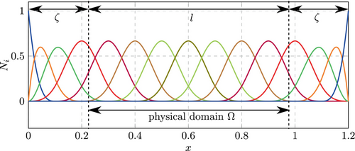
Throughout this work, we consider an elastic bar with length . No Dirichlet boundary conditions are applied, that is, both ends of the bar are free ends. The size of the fictitious domain is varied on each side according to the parameter , where . This is illustrated in Figure 2 and can be seen as a one-dimensional variant of the immersed cube considered in References 12, 13.
4.1 Frequency domain
4.1.1 Asymptotic accuracy

4.1.2 Global accuracy
4.2 Time domain
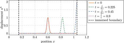
In order to assess the accuracy of the considered discretizations in the time domain, we consider two different exemplary problems.
4.2.1 Wave propagation
4.2.2 Impact problem
| Young's modulus | Density | Yield stress | Hardening coefficient |
|---|---|---|---|
| GPa | kg/m | kPa |

For the numerical investigations, a time interval of s is considered in combination with the non-zero initial velocity m/s and a penalty factor of . Figure 5 (middle) shows the resulting displacement of the right end of the bar over time for a boundary fitted setting (, ) and an immersed setting (, ). The results were obtained using a discretization based on B-splines with and a consistent mass matrix, knot spans and a time step size of s. They will be used as a reference solution for the numerical investigation. It is noted that no numerical damping was applied in this simulation. The kinetic energy is only dissipated due to the elastoplastic material behavior.
5 RESULTS: CONSISTENT MASS MATRIX
In this section, we investigate the behavior of the different discretization strategies using a consistent mass matrix. Before reporting about the accuracy in the frequency domain in Section 5.2 and in the time domain in Section 5.3, we study the influence of the fictitious domain size on the largest eigenvector. This adds to the findings from References 12, 13, where this was done for a lumped mass matrix only.
5.1 Largest eigenvalue
We revisit this study in Section 6, where we report the results obtained with a lumped mass matrix, which reproduces the results from References 12, 13. This leads to the promising bounded largest eigenvalues discovered therein. Here, we first investigate whether this is also the case for a consistent mass matrix.
5.1.1 continuous splines
Figure 6 shows the results obtained for continuous splines. Interestingly, the unstabilized case, where , yields maximum eigenvalues that approach infinity as the support of an element approaches zero, while the stabilized case yields maximum eigenvalues that only approach infinity for . As is increased, the maximum eigenvalue shows a qualitatively comparable behavior to the unstabilized case with a lumped mass matrix as investigated for an immersed cube in References 12, 13 and considered here in Section 6 (see Figure 7, top left). Quantitatively, however, the values are much higher compared to the computations with a lumped mass matrix.


5.1.2 Lagrange polynomials
Figure 7 shows the results obtained using Lagrange polynomials. Here, the eigenvalues approaches infinity as the support of an element approaches zero. This happens independently of the stabilization with . This renders standard discretizations based on Lagrange polynomials inapplicable for the solution of general immersed dynamics problems with an explicit time integration scheme. The critical time step size would become infinitely small whenever infinitely small supports arise, which for complex problems cannot be avoided a priori. Of course, remedies against this exist and an overview of the most promising ones is given in Section 7. However, to the best of the authors knowledge, an elegant strategy that results in a method with a comparable efficiency even for problems, where almost all elements are cut by an immersed boundary is not yet available.
5.1.3 Lower continuity splines

Still, for all bounded scenarios, the largest eigenvalue is found to be larger than that observed for splines with maximum continuity (see Figure 6) and far from the results observed in combination with lumped mass matrix in Section 6.
5.2 Frequency domain
In this section, the results of the investigations regarding the spectral accuracy for the different discretization schemes in combination with a consistent mass matrix is presented.
5.2.1 Asymptotic accuracy
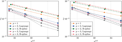
The asymptotic accuracy for Lagrange and B-spline shape functions has been investigated in several previous studies, see, for example, References 3, 37. Accordingly, we present them here only briefly in order to provide a reference of the investigations in the immersed setting and those conducted for a lumped mass matrix in Section 6. Figure 9 shows the convergence of the sixth eigenvalue and Figure 10 shows the convergence of the corresponding eigenvector. The same behavior can be observed for any eigenvalue close to the left end of the spectrum, however, the error for lower eigenvalues quickly falls to machine precision while larger eigenvalues would call for finer discretizations. The choice of was found to suit the purpose of investigating the spectral behavior best.


Regarding the immersed setting, we set and perform an -refinement for polynomials degrees up to as for the boundary fitted case. As the number of elements is increased, the location of the cut within an element changes. Therefore, we increase in steps of 1 only to encounter all possible discretizations in the convergence study. The results are shown in Figures 11 and 12. While the error undergoes some oscillations for the coarsest discretizations, the overall convergence behavior is found to be the same as that for the boundary fitted setting. The error of the eigenvalue approximated with splines with shows some oscillations also for the finest discretizations that are considered in Figure 11. These oscillations are assumed to be a result of the finite precision arithmetic and will be encountered again for the computations performed with a lumped mass matrix in Section 6, where we address this phenomenon in more detail. Interestingly, no oscillations for fine discretizations are found for the error in the eigenvectors (see Figure 12). It is noted that for all computations, the search methods described in Section 4.1.1 was applied. For several of the encountered discretizations, and but never (the discrete eigenvalue and eigenvector that yielded the smallest error were not the sixth but always the index that yielded the smallest error was the same for the eigenvalue and the eigenvector).


5.2.2 Global accuracy
As explained in Section 4.1.2 we examine the accuracy of eigenvalues and eigenvectors of the entire discrete spectrum following the investigations from Reference 3. We evaluate the three relative errors here for a discretization with approximately 100 degrees of freedom. While for computations with splines, the number of elements is kept constant at regardless of the polynomial degree, we set for computations with Lagrange polynomials.
We start our investigation by reconsidering a well known result from Reference 3. Figure 13 shows a comparison between the global accuracy obtained for a discretization with splines and Lagrange polynomials for . The discretization with splines shows several advantages here. Firstly, the accuracy in the low end of the spectrum is much higher (for a zoom into this region, see Reference 3). Secondly, there is no so called optical branch, as observed for Lagrange polynomials (and like-wise for continuous splines) at . Thirdly, the eigenvectors associated with the largest eigenvalues obtained from the discretization with splines are localized towards the domain boundary, whereas for Lagrange polynomials, this is not the case. While this renders the spline based discretization superior with regard to the considered global accuracy, Lagrange polynomials show a lower maximum eigenvalue. For them, the relative error for so called outliers (severely overestimated eigenvalues towards the high end of the spectrum) never exceed 50%, whereas for splines, the largest two eigenvalues are overestimated by around 115%.
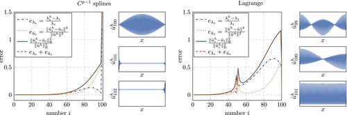
The same advantages and disadvantages are observed for , see Figure 14. Again, splines yield a much higher accuracy for almost all parts of the spectrum. The only exception is again observed for the outliers, which have a relative error of around 65% for Lagrange polynomials and around 360% for splines. Lagrange polynomials now yield two bifurcations or optical branches, one at (not well observable in Figure 14, see Reference 3 for a zoom into this region) and one at .
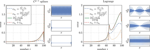
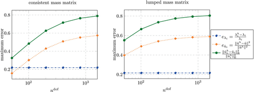
It is noted that the global relative errors–in particular in the bifurcation region at – are not converged for the chosen discretizations with . As shown in Figure 15, much finer discretizations are needed for a quantitative statement about the maximum error. However, for a qualitative analysis of the discretizations it is found that is sufficient. Further, this allows for a visual inspection of selected eigenvectors at the right end of the spectrum, which is not possible for much larger values of due to the accordingly much stronger localization towards the domain boundaries.
5.3 Time domain
In this section the results in the time domain are presented. Having observed the largest eigenvalue approaching infinity as the support of a basis function approaches zero, it is expected that very small time step sizes are needed in order to perform stable simulation with the CDM as described in Section 3.3. In addition to a pure investigation of the accuracy of the spatial discretization method this section also serves to find suitable parameters for the temporal discretization method.
5.3.1 Wave propagation
For the solution of the wave propagation problem as described in Section 4.2.1, we construct again different variants by varying the size of the fictitious domain . Different than in Section 5.1, we choose finer discretizations with an approximately equal number of degrees of freedom. This is achieved by choosing the number of elements (knot spans) to be , where for Lagrange polynomials and for B-splines . Lower continuity splines are not considered here. The range in which varies is modified accordingly, such that elements (knot spans) lie completely in the fictitious domain if reaches its maximum. Considering the fact that the number of elements for is increased by a factor of 20 compared to the investigations from Section 5.1, this is done by dividing the values for defined in Equation (25) by 20. The wave propagation problem is then solved using either or an approximately constant , which is chosen such that the simulations are stable for all considered values of and such that the desired end time is (where the wave is expected to arrive back at the center of the bar).
Figure 16 shows the largest eigenvalues and the error obtained for . Qualitatively, the largest eigenvalue behaves equivalently to the study with a constant number of elements (see Figures 6-8). As the support of an element (a knot span) approaches zero, approaches infinity. Different than before, this happen four times for B-spline discretizations (independent of the polynomial degree) and times for Lagrange discretizations due to the choice for a fixed number of degrees of freedom and the accordingly different number of elements. It is obvious that the error shown in Figure 16 (right) is dominated by the time step size, which is indicated therein as well. Only for a discretization with quadratic Lagrange polynomials, the error does not directly follow the values for , which indicates that the spatial discretization error dominates here. Before considering the results obtained with an approximately constant , which confirm this assumption, a close look needs to be taken at the results obtained for a discretization with cubic Lagrange polynomials.
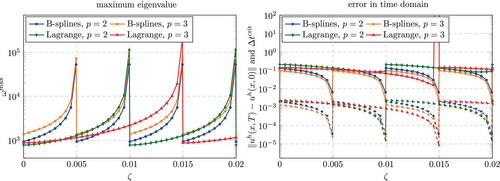
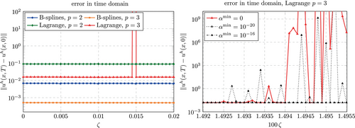
From Figure 16 (left), it can be seen that this discretization yields an extremely large error () for , which corresponds to an immersed boundary that cuts an element such that only lies inside the physical domain. It results from unphysical oscillations that initiate in the fictitious domain and increase drastically once the wave reaches the immersed boundary. This is illustrated in Figure 17 (left) for the a time step size of . Interestingly, the error increases, if the time step size is decreased as shown in Figure 17 (right). Decreasing even further, the unphysical oscillations reach large values even before the wave is reflected at the immersed boundary. However, it is emphasized that these oscillations can be counteracted by a stabilization with a non-zero value for . Setting already suffices to completely eliminate the oscillations without increasing the error to a noticeable extend. We will give a quantitative overview on the effects of such a stabilization for the simulations using am approximately constant time step size presented in the following.

From Figure 16 (left) it can be seen that for , a time step size of and for a time step size for is sufficient to obtain stable simulations for all considered values of . In order to include the desired end time mentioned above, we chose and , respectively. The results for all considered discretizations are shown in Figure 18 (left). As expected from the asymptotic accuracy, the B-spline discretizations yield a significantly lower error compared to the discretizations based on Lagrange polynomials. Interestingly, the error is almost unaffected by the size of the fictitious domain for all discretizations. Again, an exception is found for cubic Lagrange polynomials in combination with . In order to investigate this phenomenon in more detail, Figure 18 (right) shows the error obtained for values of in this critical region. It includes the results obtained using and confirms that this stabilization is sufficient to obtain results in the same region as those obtained for cubic Lagrange shape function outside of the critical region ( in the critical region, in the range from Figure 18 (left) excluding ). The results for and in Figure 16 (right) show that the simulation becomes unstable for certain values of . Interestingly, this is not the case from a certain value on, where the support of the cut element falls below a certain percentage. Instead, several values yield stable simulations also for smaller supports that the one, for which an instability is first observed (). For smaller values of , no instabilities could be observed.
5.3.2 Impact problem
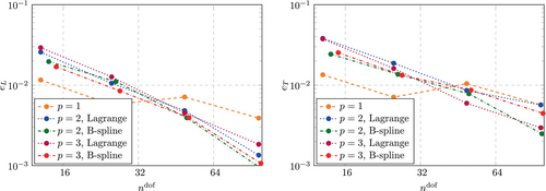
The impact problem introduced in Section 4.2.2 is computed using the strong and weak formulation of the contact with the rigid wall. To begin with, the boundary fitted setting () is considered. Figure 19 shows the results obtained for the strong setting and coarse discretizations with . While the displacement is underestimated for Lagrange polynomials and B-splines, the results are very close to the reference solution. The only difference between the two types of shape functions is observed for the plastic strain, which is much smoother and closer to the reference solution for B-splines (Figure 19 (right) shows the plastic strain values at the quadrature points).

Figure 20 shows the convergence behavior under mesh refinement for the boundary fitted case. Clearly, non of the discretizations yields a high-order convergence as expected for smooth problems and observed before in the frequency domain. This is attributed to the nature of this problem, which is non-smooth due to the elastoplastic material behavior as well as the impact itself. Accordingly, it is expected that the effects due to lumped mass matrices and immersed boundaries are different than those observed in the frequency domain and the wave propagation problem in the time domain.
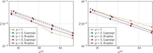
The same convergence study is also performed in the immersed setting. In order to leave the length of the bar unchanged at , we chose and . The results in Figure 21 differ only marginally from those in Figure 20, that is, the impact of the immersed boundary on the accuracy is negligible. However, as observed before, the critical time step size is affected. In fact, all simulations with had to be done with a smaller time step size than the default value of . In these cases, the time step size was set to and the error measure (see Equation 24) is computed based on a linear interpolation of the solution at the resulting time steps.
6 RESULTS: LUMPED MASS MATRIX
In this section, we report the results obtained with lumped mass matrices. The structure follows again that of Section 5, that is, we first show investigations of the influence of the fictitious domain size on the largest eigenvalue and then consider the accuracy in the frequency domain (Section 6.2) and the time domain (Section 6.3).
6.1 Largest eigenvalue
In this section, we repeat the study from Section 5.1, where we vary the fictitious domain size and observe the largest eigenvalue for a coarse discretization with elements or knot spans, respectively. This directly corresponds to a one-dimensional variant of the immersed cube considered in References 12, 13. In addition to the studies therein, we include Lagrange polynomials here and investigate the influence of stabilization.
6.1.1 continuous splines
The results for continuous splines are shown in Figure 22 (left) for the unstabilized case and found to be equivalent to the results in three dimensions from References 12, 13. Remarkably, the largest eigenvalue is bounded and significantly reduced if and the outer knot spans lie completely in the fictitious domain. Considering the efficiency of explicit time integration schemes like the CDM, this renders the immersed setting favorable over the boundary fitted setting. For the stabilized case shown in Figure 22 (right), the advantage is not as surprising in view of the fact that the eigenvalue is also bounded for a consistent mass matrix (see Figure 6). However, quantitatively, both cases shown in Figure 22 constitute a profound improvement to the stabilized case with a consistent mass matrix. Of course, this improvement is to be seen only with regard to the largest time step size achievable with explicit time integration schemes and not with regard to the accuracy of the methods, which is addressed in Sections 6.2 and 6.3.

6.1.2 Lagrange polynomials
Figure 23 show the results obtained for Lagrange polynomials. Here, lumping does not lead to the desired boundedness of the largest eigenvalue. As was observed for the corresponding investigations with a consistent mass matrix (see Figure 7), it was found that the stabilization has no noticeable effect, such that we restrict us here to the unstabilized case3. However, a difference is found with respect to the applied lumping scheme. For row summing, the largest eigenvalue remains acceptably low for a wider range of fictitious domain sizes, while for HRZ lumping the divergence initiates earlier.

6.1.3 Lower continuity splines
For splines, the same behavior reported in References 12, 13 for the unstabilized case is observed for both cases, see Figure 24. As approaches the position of a knot (multiples of 0.1), the largest eigenvalue diverges. While it is found to be lower than that observed for Lagrange polynomials if at least 50% of the knot span is in the physical domain, the divergence behavior is comparable to that observed for Lagrange polynomials combined with row summing. Overall, it is noted that changes in lead to smooth and monotonic changes in the largest eigenvalue despite the large steps of around 0.01, whereas for Lagrange polynomials, the changes show oscillations.

6.2 Frequency domain
In this section, we repeat the study from Section 5.2, starting with an investigation of the asymptotic accuracy, followed by an investigation of the global accuracy.
6.2.1 Asymptotic accuracy
As before, we split the studies of the asymptotic accuracy into two parts, considering the boundary fitted setting first, followed by the immersed setting.
Boundary fitted setting
Figure 25 shows a comparison between the convergence behavior of the sixth eigenvalue obtained with continuous splines and that obtained with Lagrange polynomials. The fact that the accuracy is reduced to second order for splines independently of the polynomial degree is well known and was previously reported in Reference 37 and further investigated in Reference 3.
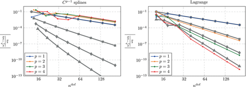
- The considered lumping schemes (row summing, HRZ lumping) are equivalent to a nodal quadrature for the considered case of one-dimensional elements with equidistant interconnecting nodes as shown in Reference 10. Therefore, the present discretization correspond to the spectral element method, which generally results from a nodal quadrature.
- The accuracy of eigenvalues computed by the spectral element method is times higher than that of the classical finite element method with a consistent mass matrix as shown in Reference 5.
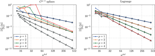
Considering the predicted eigenvectors, the reduction of the accuracy due to lumping is not as severe as for the eigenvalues for splines as shown in Figure 26. For Lagrange polynomials, the accuracy is not affected by lumping.
Immersed setting
Proceeding with the immersed setting, we perform again convergence studies, where the number of elements is increased in steps of 1 in order to encounter any possible discretization of the immersed bar problem at hand. In fact, this particular study has led us to such a fine grained analysis, which reveals unexpected oscillations in the error regarding eigenvalues as well as eigenvectors.
The convergence behavior of the eigenvalues is shown in Figure 27. The behavior for continuous splines is as expected, namely converging with second order, independent of the polynomial degree. Occasionally, the error is lower than this general trend, which is explained by the search method described in Section 4.1.2 that will always pick the eigenvalue from the discrete spectrum that yields the lowest error. For Lagrange polynomials, the orders and yield again the same and a higher accuracy, respectively, than that obtained for a consistent mass matrix, however, oscillations are clearly visible for . For , the trend of a higher accuracy compared to the results for a consistent mass matrix is barely recognizable. Only occasionally, the error is as low as expected from the boundary fitted setting, while for most discretizations, the error is unexpectedly large. At this stage, one may be tempted to attribute this behavior to negative entries in the diagonal of the mass matrix, that may arise from the row summing technique. However, we have found no correlation between the number of negative diagonal entries and the oscillations seen in Figure 27. Instead, we assume that a bad conditioning of the system matrices in combination with finite precision floating point arithmetics causes this issue. We will come back to this at the end of this section, after considering the convergence behavior of the eigenvectors, which shows even larger oscillations.
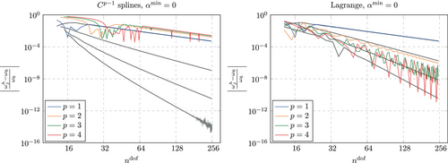
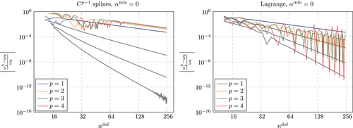
In fact, the predicted eigenvalues for both types of shape functions, splines as well as Lagrange polynomials can no longer be called converging as shown in Figure 28. Instead, unpredictable spikes of large errors appear for certain discretizations, as the mesh is refined and the location of the immersed boundary with respect to the element boundary changes. These oscillations are more pronounced for Lagrange polynomials than for splines.
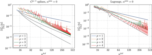
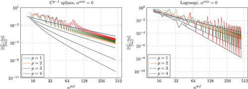
As mentioned above, HRZ lumping can be considered the more natural lumping scheme for Lagrange polynomials because it avoids negative diagonal entries. Therefore, we also show the results obtained with this method in Figures 29 and 30 and for completeness include again discretizations based on splines. However, the qualitative behavior remains the same as that observed for row summed mass matrices. Quantitatively, it is observed that the magnitude of the oscillations in the eigenvector error is even increased for Lagrange polynomials.
- Residual of the eigenvalue problem
- Number of negative eigenvalues
- Number of complex eigenvalues
- Condition number of and
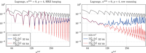
All of these quantities indicate that the system is badly conditioned and results in spurious modes, however, none of these quantities correlates with the oscillations seen in Figures 27-30. Concluding, we have to say that alternative eigenvalue solvers or higher precision arithmetics are needed in order to accurately solve for the eigenvalues in the immersed case. We have used the NumPy38 implementation of ARPACK,39 which can be seen as the state-of the art for this type of problems. Further, we compared the results to those obtained using MATLAB's function eigs (see Reference 40) for selected discretizations and observed the same inaccuracies.
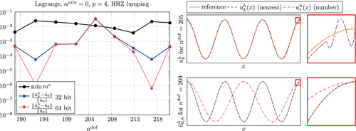
While the results obtained with row-summed mass matrices (Figure 31 (right)) indicate that the oscillation can be explained by the finite precision arithmetics (possibly alone), the results obtained with HRZ lumping (Figure 31 (left)) indicate that in particular the maxima in the error observed for certain discretizations have another origin and might be inherent to the system. To provide more insight into this phenomenon, Figure 32 shows a close zoom into a selected range of degrees of freedom in combination with the eigenvectors that were approximated most inaccurately. We will revisit in particular the discretization with again in Section 6.3.1 and investigate how the large error observed here effects the accuracy of simulations in the time domain.
6.2.2 Global accuracy
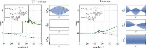
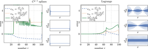
Having observed the severe oscillations in the accuracy of the eigenvectors for the low end of the spectrum in the immersed setting, which seem unpredictable without further investigations, we restrict our study of the global accuracy to the boundary fitted case. Considering the different effects of lumping on spline discretizations and discretizations based on Lagrange polynomials, a major difference in the global accuracy is expected as well. It is noted that no search method for eigenvalues or eigenvectors is performed for the global accuracy studies.
Spurious eigenvectors
In order to further investigate what happens at the discontinuity, we show in Figure 35 the eigenvectors in this region of the spectrum for a consistent mass matrix and compare it with the eigenvectors obtained with the lumped mass matrix shown in Figure 36. Having observed the discontinuity around (cf. Figure 13) we include the eigenvectors for in Figure 35. While there is almost no visible difference between the approximated and the exact solution for B-splines, Lagrange shape functions yield eigenvectors which have no approximability whatsoever. This loss of approximability starts to show already for modes further below the discontinuity, which is why Figure 35 includes also eigenvalues for . It is worth noting that the error in the eigenvalues seems to arise because a low frequency oscillation is introduced, which makes the eigenvector inaccurate throughout the entire domain and not only in a localized region as observed for the outliers before.
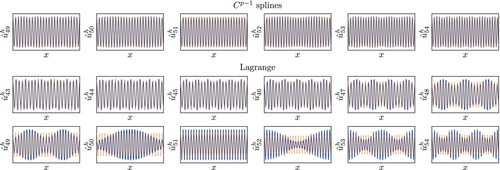
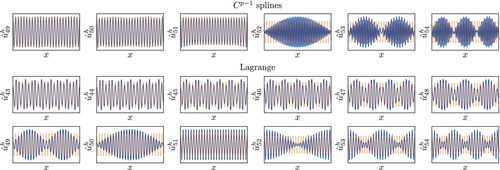
Considering the same range of eigenvalues obtained with a lumped mass matrix, see Figure 36, also the B-spline discretization looses its approximability. However, a discontinuity is also visible for the eigenvectors, that is, the error suddenly increases at , whereas for Lagrange shape function the increase is more gradual.
Two more interesting aspects can be seen from Figures 35 and 36. Firstly, also the accuracy of Lagrange shape functions is affected by lumping–the lower modes in the considered range become less accurate. Secondly, a qualitative difference between Lagrange shape functions and B-splines can be observed for the error of the higher modes in the considered range. While for Lagrange shape functions, the eigenvectors seem to be composed out of a low frequency and a frequency that matches that of the exact eigenvector, B-splines yield eigenvectors that seem to be composed of a low frequency and a high frequency, which is higher than that of the exact eigenvector.
6.3 Time domain
In this section, we report about the results obtained with lumped mass matrices for the problems introduced in Section 4.2.
6.3.1 Wave propagation
Considering the wave propagation problem, we investigate again the effect of the fictitious domain size on the largest eigenvalue and the accuracy. Apart from lumping the mass matrices using row-summing for B-splines and HRZ lumping for Lagrange polynomials, we use the same discretizations as for the studies using a consistent mass matrix in Section 5.3. Summarizing, this means we vary the fictitious domain size in the same manner and construct discretizations with approximately 240 degrees of freedom . Further, we consider to sets of simulations, one with a time step size of and one with time step sizes of (for ) and (for ).
The results obtained with are shown in Figure 37. For Lagrange polynomials, the results are very similar to those obtained with a consistent mass matrix (see Figure 16). The largest eigenvalues approaches infinity as the support of an element approaches zero and the error is dominated by the temporal discretization error. Interestingly, no instability is observed for the previously identified critical values of . For discretizations based on B-splines, the spatial discretization error dominates. Due to the loss of accuracy that results from lumping the mass matrix, the error is found to be independent of the fictitious domain size and comparably large (). As expected from Section 6.1, the largest eigenvalue is bounded and much lower than that obtained for Lagrange polynomials.
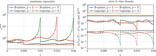
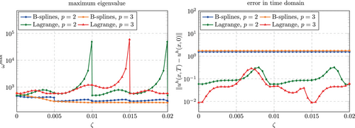
Figure 38 shows the results obtained using an approximately constant time step size. The error for the considered B-spline discretizations is again independent from the fictitious domain size and its magnitude does not change noticeably compared to the simulations with . For Lagrange polynomials, the results are significantly affected by and vary over more than one order of magnitude (). Interestingly, there seems to be a weak spot, when approximately 20% (for ) or 40% (for ) of an element lies inside the physical domain (for and () and for ()). Here the error rises by about half an order of magnitude. On the other hand, if the elements have at least 50% support in the physical domain, the error is lower than that observed for a consistent mass matrix.
Finally, we reconsider the discretization using Lagrange polynomials and HRZ lumping with , which was identified to have an unexpectedly low accuracy in the predicted eigenvector (see Figure 32). Snapshots of the solution to the wave propagation problem based on a discretization with are shown in Figure 39. Considering the full range of displacement an increase in the error compared to the reference solution is hardly visible but the zoom towards the -axis in Figure 39 (right) highlights the spurious oscillations. The error is within the range found for quadratic and cubic Lagrange polynomials in Figure 38.

6.3.2 Impact problem
So far, the effect of lumping and immersed boundaries on the accuracy of a discretization was investigated for smooth problems. This allowed for high-order convergence rates according to the polynomial degree of the shape functions–with the exception of B-splines in combination with lumping as well as Lagrange polynomials in combination with certain immersed boundary locations and lumping.
Conversely, the solution of the impact problem introduced in Section 4.2.2 and addressed using consistent mass matrices in Section 5.3.2 is not smooth and the convergence rates are limited. Accordingly, for this exemplification of an application-oriented problem, the impact of lumping may not be as significant, which initially motivated this study.
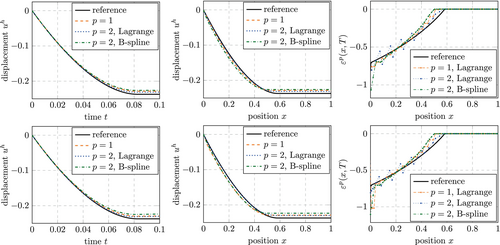
Figure 40 shows the displacement solution obtained for different discretization and lumped mass matrices. Comparing the displacement results for the boundary fitted setting (top row in Figure 40) with those presented in Section 5.3.2, only a moderate increase in the deviation from the reference solution is observed. A further but again moderate increase is observed in the immersed setting (bottom row in Figure 40). More severe deviations are observed for the plastic strain in the impact region. Here, lumping leads to overestimations, which occur independently of the type of shape functions in the immersed setting and occur only for B-splines in the boundary fitted setting. This trend continues for larger polynomials degrees , which where excluded in the presentation for clarity.
As before, we consider the convergence of the error measures and , referring the displacement of the right end of the bar () over time and the displacement within the bar at the time , respectively. The results obtained for the boundary fitted setting are shown in Figure 41. The lumping increases the error significantly, however, the convergence order is unchanged. Figure 42 shows the results obtained in the immersed setting. Like before the case and is considered such that effectively the same problem is solved. The increase in error is qualitatively and quantitatively very similar to that in the boundary fitted setting. Interestingly, the lumping increased the critical time step size to such an extend that all results could be obtained using the default time step size for this problem of . As indicated in Figure 42 and mentioned in Section 5.3.2 this was not the case for the simulations with consistent mass matrices.

7 SPECIAL TECHNIQUES
In this section, we consider some remedies against the loss of accuracy observed for B-splines in the case of mass lumping and against the diverging largest eigenvalue for Lagrange polynomials in case of badly cut elements.
7.1 Interpolatory spline basis

7.2 Eigenvalue stabilization
In order to overcome the problem of large eigenvalues in badly cut Lagrange elements, a stabilization techniques that goes back to Reference 41 and was already successfully applied to nonlinear static analyses (see Reference 42) is a promising remedy. We apply it here in a very simple form with the intend to show the general applicability of the method in the context of explicit dynamic analyses. For an in depth study of the opportunities and limitations of the method, we refer the reader to Reference 43.
While several more sophisticated heuristics have been introduced in References 41-43 to compute a different for each mode and to do so in a way that the stabilization method becomes independent of chosen material, we use a constant value of here. The threshold is set to . It is further noted, that the stiffness matrix may be stabilized as well, however, physical rigid body modes, which are associated with zero eigenvalues must be identified and excluded from . While this is a trivial task for one-dimensional problems, an orthogonalization procedure needs to be applied in higher dimensions. For the present study of the general applicability, we have found that stabilizing the mass matrix is sufficient for the desired increase of the critical time step size.
7.3 Frequency domain: Asymptotic and global accuracy
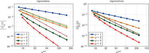
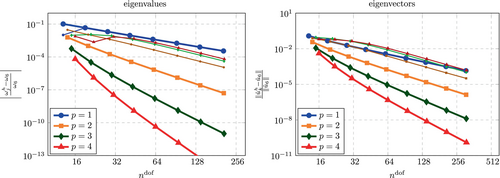
In order to investigate the properties of the interpolatory basis functions, we consider again the asymptotic and global accuracy. Figure 44 shows the convergence for the eigenvalues and eigenvectors. Compared to the standard spline basis (see Figures 9 and 25), the accuracy is much less affected by lumping. For a consistent mass matrix, the convergence behavior is equivalent to that of the standard spline basis, which is expected because the two basis span the same space. For completeness, Figure A3 shows the results obtained for the same study but using the HRZ lumping technique. While the accuracy is not as high as for row-summing, it is still considerably better than for standard splines (see Figure A2).
As shown in Figure 45, also the global accuracy is much less sensitive to lumping using the row-summing technique. For , no bifurcation is observed and the accuracy is comparable to that achieved for Lagrange polynomials, while the eigenvalues are slightly less accurate and the eigenvectors are slightly more accurate (cf, Figure 33). For , a bifurcation is observed, beyond which the accuracy of the eigenvectors deteriorates. However the bifurcation is shifted far towards the high end of the spectrum, as opposed to the results for the standard spline basis (cf, Figure 34). For the HRZ lumping techniques, an equivalent global accuracy is observed, see Figure A4. For a consistent mass matrix, the global accuracy is indistinguishable from the the one obtained for the standard spline basis as shown in Figure A5.

Accuracy of selected eigenvectors
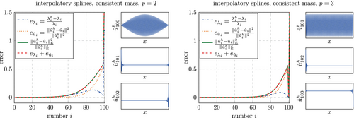
As expected from Figure 45, the eigenvectors obtained with the interpolatory splines are accurate also in the region where a bifurcation was observed for Lagrange elements in general and for B-splines in combination with lumping. This can be seen Figure 46 which shows the eigenvectors in the region, where the bifurcation was observed before ( for ).

Of course, for the interpolatory spline basis, the eigenvectors around its bifurcation point at observed for are of interest as well. They are shown in Figure 47. Again it can be observed that the inaccurate eigenvectors contain not only the frequency of the exact one but at least one more frequency. Further, the accuracy in the considered region is comparably low even for the consistent mass matrix, which is to be expected given the fact the region is lying close to the right end of the spectrum (Figure 47 shows the eigenvectors 83 to 88 out of 103).

We do not consider the eigenvalue stabilization technique in the frequency domain and refer the reader to Reference 43, where it is investigated in detail.
7.4 Time domain: Wave propagation
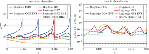
In this section, computations in the time domain are presented. We consider only the wave propagation problem described in Section 4.2.1. The fictitious domain size is changed in the same way as for the investigations in Sections 5.3.1 and 6.3.1. Figure 48 shows the results obtained for selected discretization methods with a polynomial degree of and without stabilization (). In order to summarize the results obtained with the standard technique and to provide a reference the standard discretization techniques are included in Figure 48 as well.
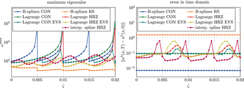
As described before, the standard spline basis combined with a row-summed mass matrix yields very low maximum eigenvalues, however, the accuracy is worse than for all other methods. Splines with a consistent mass matrix yield the most accurate results, however, as the support of a basis function approaches zero, the maximum eigenvalue approaches infinity (for , , , ). Lagrange polynomials yield a diverging maximum eigenvalue when the support of an element approaches zero (for , ) for lumped and consistent mass matrices. The accuracy for the consistent mass matrix is acceptable as expected, however, much lower than that achieved for splines. The accuracy is influenced by lumping and the influence depends on the location of the cut, that is, where the immersed boundary intersects the element.
The interpolatory spline basis combined with a consistent mass matrix could not be applied for all values of . Whenever the immersed boundary coincides with a knot () the central difference method showed instabilities. This combination is therefore omitted in Figure 48. The interpolatory spline basis combined with the HRZ lumping technique yields the desired results of a low largest eigenvalue and an acceptable accuracy at the same time. While the eigenvalue is higher compared to the standard spline basis combined with a row-summed mass matrix and the accuracy is only in the range observed for Lagrange polynomials, it still constitutes a very promising method for problems solved with an explicit time integration scheme. However, further studies need to investigate the effect of the global support of the basis function on the computation time. While the mass matrix is diagonal due to the lumping and the solution of the linear system (8) reduces to a component-wise vector multiplication, the computation of the right hand side involves a matrix-vector multiplication with a fully populated stiffness matrix, which may slow done the solution process significantly.
The discretizations based on Lagrange polynomials with eigenvalues stabilization (EVS) perform similarly well. Comparing the largest eigenvalue and the error in Figure 48 with those obtained for classical Lagrange polynomials, one can detect where the EVS was active, namely for and , independently of the employed mass matrix. For the consistent mass matrix, the largest eigenvalue is larger than that found for the interpolatory spline basis but the error is lower. For a mass matrix with HRZ lumping, the largest eigenvalue is lower but the error is increased to the same level observed for the interpolatory spline basis.
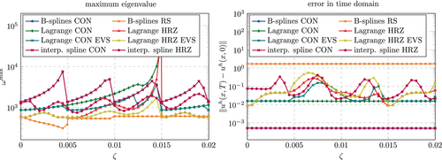
Figure 49 shows the corresponding results for the stabilized case (). With this setting, also the interpolatory spline basis can be combined with a consistent mass matrix and yields identical results to those obtained with the standard spline bases. As before (see Figures 6 and 8) it is observed than the largest maximum eigenvalues is bounded for both of these discretization. The discretizations based on Lagrange polynomials with EVS are not noticeably influenced by the -stabilization.
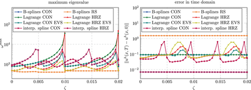
Figures 50 and 51 show the results of the same investigation performed for cubic shape functions. The same trend is observed here as well. Again, discretizations that lead to instabilities in for any of the considered values of were discarded from the plots. This only happens for Lagrange polynomials and interpolatory splines in combination with a consistent mass matrix in the unstabilized case shown in Figure 50. Comparing again the eigenvalue stabilization with the interpolatory splines, a similar behavior is observed as before for . The EVS combined with a consistent mass matrix yield lower errors but larger , while the EVS combined with a lumped mass matrix yield larger errors but lower .
7.5 Further techniques
In this section, we would like to refer to alternative remedies that realize a diagonal mass matrix for discretizations based on B-splines without a severe loss in accuracy or increase the critical time step size to an acceptable level for discretizations based on Lagrange polynomials.
We would also like to mention polynomial extension as a remedy against large eigenvalues resulting from badly cut elements. It was investigated in several publications in the context of isogeometric analysis, most recently in References 47-50. While the issue of badly cut elements, respectively badly trimmed knot spans, can be counteracted by sufficiently large fictitious domains in case of B-spline discretizations (as discovered in Reference 13), the polynomial extension may also be applied in case of Lagrange discretizations. The basic idea is to extend basis functions of neighboring elements into the badly cut element and partly or entirely removing the basis function of the badly cut element from the discretization.
So called ghost penalty and ghost mass methods provide yet another way to circumvent the strict requirements on the time step size. They were investigated recently in the context of IGA in Reference 51. Both strategies add a term to the weak form that penalizes jumps in the derivatives of the shape functions across element boundaries. An advantage of these methods is that shape functions remain unaltered. However, the resulting system matrices are not amendable to classical lumping schemes.
Besides the eigenvalue stabilization summarized in Section 7.2, several other strategies that circumvent the requirement of a very small time step size were investigated in the context of Lagrange polynomials. This includes modified time integration schemes, in particular implicit-explicit (IMEX) schemes, where the elements which are badly cut are treated using an unconditionally stable implicit scheme, while the conditionally stable explicit scheme is used for the uncritical elements. An alternative are Leapfrog algorithms, which in this context effectively realize smaller time step sizes for the critical elements, while in uncritical elements a larger time step size is kept. Preliminary investigations on these methods have been presented in Reference 52. More recently, the application of IMEX schemes for immersed boundary value problems was investigated in more detail in Reference 11. Such time integration schemes have been established previously outside of the context of immersed methods, see, for example, References 16, 17, 53.
As shown in the comparisons of the accuracy for the different discretizations in Sections 6.3 and 7.4, Lagrange basis function do not only suffer from large eigenvalues due to cells with small support. They also show a decreased accuracy for unfortunate locations of the cut, for example, when approximately of a quadratic or of a cubic element lies in the physical domain (see Figures 38, 48 and 49). Incomplete lumping is an interesting and very simple remedy against this. The idea is to lump only uncut elements, which lie completely inside the physical domain. If the number of cut elements is moderate, this leads to almost diagonal mass matrices that can be factorized considerably faster than the consistent mass matrices obtained without any lumping. In order to circumvent the strict requirements on the time step size, IMEX schemes as in Reference 52 or eigenvalue stabilization methods as in Reference 43 can be applied.
8 SUMMARY AND CONCLUSION
- The largest eigenvalue for B-spline discretizations is also bounded when a consistent mass matrix is used in combination with -stabilization, that is, using . While it is much larger than with row-summed mass matrices, this still constitutes an advantage compared to the diverging largest eigenvalue observed for -continuous discretizations.
- The global accuracy of eigenvalues and eigenvectors predicted by B-spline discretizations (boundary-fitted or immersed) shows a discontinuity at the mode number (as opposed to the well known optical branches of -continuous discretizations starting at ).
- In the immersed setting (with and without lumping), both types of discretization lead to spurious modes, whose eigenvalues do not take extreme values but lie close to physical modes.
- In the immersed setting and with lumped mass matrices the asymptotic accuracy of both types of discretization depends on the position of the cut. For Lagrange polynomials, this effect is more severe than for B-splines, and an -refinement study, for which the cut changes its location within an element, may not yield converging eigenvalues.
- Interpolatory spline bases which span the same space as classical B-spline bases can effectively reduce the loss in accuracy due to lumping. While the interpolatory basis proposed in References 24, 27 yields this desired effect, the support of the basis functions is global.
- An eigenvalue stabilization technique can effectively decrease the largest eigenvalue for Lagrange discretizations. However, an extension to two and three spatial dimensions is not straight-forward and optimal parameters still have to be determined.
Concluding, we can state that mass lumping applied to classical B-spline discretizations must be taken with care. While it leads to bounded largest eigenvalues without further stabilization, the accuracy is diminished. In the boundary-fitted setting, at least an asymptotic convergence of reduced order was previously determined for eigenvectors. However, this is not guaranteed in the immersed setting for , where the accuracy depends on the location of the immersed boundary. Also the global accuracy is reduced due to spurious modes entering the discrete spectrum even in the boundary-fitted setting. An effect of these phenomena on the accuracy of computations in the time domain is clearly present, in particular for the considered wave propagation problem. For the considered impact problem with plastic material behavior, the effect is less pronounced. As a whole, the results show that consistent mass matrices in combination with classical -stabilization might be considered as an alternative to lumping for B-spline discretizations. Due to the extremely high accuracy per degree of freedom and a bounded largest eigenvalue due to the stabilization, the resulting simulation can be more efficient than one with a lumped mass matrices that yields the same accuracy. This shifts computational cost from the evaluation of the right hand side vector (which has to be done in every time step) to the factorizing the mass matrix (which has to be done only once). Accordingly, it depends on the underlying problem which mass matrix yields the most efficient method. Of course, all of the above concerns assume that none of the mentioned promising special techniques such as interpolatory and dual bases are available.
Further, we can state that mass lumping applied to classical discretizations based on Lagrange polynomials in an immersed setting must be taken with care. While lumping may even increase the accuracy in a boundary-fitted setting, it leads to a severe drop in the asymptotic accuracy that strongly depends of the location of the immersed boundary for . This effect is much stronger compared to the similar effect observed for B-splines. In particular the accuracy of predicted eigenvectors is reduced by this, but also the eigenvalues become less accurate. In contrast, the global accuracy in the boundary-fitted setting is almost unaffected by lumping for Lagrange polynomials. While the above concerns about the asymptotic accuracy make an efficient analysis in the frequency domain questionable, the accuracy of computations in the time domain seem to be rather unaffected by lumping and only moderately dependent on the location of the immersed boundary. Further, simple strategies to restore the accuracy such as incomplete lumping are readily available and lead (depending on the geometric complexity) to almost diagonal mass matrices. These can be factorized much faster than fully consistent mass matrices. However, the unbounded largest eigenvalue makes a direct application of conditionally stable time marching schemes impossible. This issue cannot be resolved by the classical -stabilization. Accordingly, discretizations based on Lagrange polynomials (with lumped or consistent mass matrix) cannot be applied directly in an immersed setting using explicit time marching schemes. If very small time steps are required by the physics of the problem, a simple remedy may be to delete elements with a very small support that would otherwise yield even smaller time step sizes. Generally, however, special techniques such as eigenvalues stabilization or ghost penalty methods are useful.
Finally, it can be said that investigations and further development of the special techniques for both Lagrange polynomials and B-splines is regarded as very important based on the findings in this work. The results presented here can help in this process and promote the consideration of all aspects taken into account here, namely asymptotic accuracy, global accuracy, and accuracy and stability in the time domain. The ongoing research in the field has already brought forth promising techniques that make an efficient and accurate explicit discretization method with a diagonal mass matrix seem in reach. The existence of a single method to suit all problems is unrealistic. It is therefore just as important to study the existing methods and special techniques in the context of larger scale applications. Many engineering problems show characteristics, for example, non-smoothness, that prevent optimal convergence of classical high-order methods. In such cases the drop in accuracy observed for lumping in the immersed setting may not be of concern. The impact problem with plasticity is a simple example that shows this trend.
ACKNOWLEDGMENTS
The authors gratefully acknowledge the support of the DFG (Deutsche Forschungsgemeinschaft) under DU 405/20-1 (grant number 503865803). A. Reali, G. Sangalli, and M. Torre acknowledge the support of the Italian Ministry of University and Research (MUR) through the PRIN project COSMIC (No. 2022A79M75), funded by the European Union–Next Generation EU, as well as the contribution of the National Recovery and Resilience Plan, Mission 4 Component 2–Investment 1.4–National Centre for HPC, Big Data and Quantum Computing, spoke 6. A. Reali and G. Sangalli are members of the Gruppo Nazionale Calcolo Scientifico-Istituto Nazionale di Alta Matematica (GNCS-INDAM), and also acknowledge the support of the Italian Ministry of University and Research (MUR) through the PRIN 2022 PNRR project NOTES (No. P2022NC97R), funded by the European Union–Next Generation EU.
ENDNOTES
APPENDIX



Open Research
DATA AVAILABILITY STATEMENT
The data that support the findings of this study are available from the authors upon reasonable request.


