CutFEM: Discretizing geometry and partial differential equations
Summary
We discuss recent advances on robust unfitted finite element methods on cut meshes. These methods are designed to facilitate computations on complex geometries obtained, for example, from computer-aided design or image data from applied sciences. Both the treatment of boundaries and interfaces and the discretization of PDEs on surfaces are discussed and illustrated numerically. Copyright © 2014 John Wiley & Sons, Ltd.
1 Introduction
Research in numerical methods for solving problems in science and engineering has mainly focused on techniques for approximating models described by partial differential equations (PDEs), while the important coupling to the geometrical description of the domain has been largely overlooked. In recent years, the need for a unified approach has been recognized, and this area is today receiving rapidly increasing interest. This interest is motivated by the demand for efficient and robust techniques for solving problems involving complex and evolving geometries. The use of geometric descriptions in the computational method, that are closely linked to the geometric data acquisition, can dramatically reduce the computational cost of preprocessing, or transformation, of acquired geometry descriptions into representations suitable for the computational method at hand.
For instance, the simulation of blood flow dynamics in vessel geometries requires a series of highly non-trivial steps to generate a high quality, full 3D finite element mesh from biomedical image data 1. Similar challenging and computationally costly preprocessing steps are required to transform geological image data into conforming domain discretizations, which respect complex structures such as faults and large scale networks of fractures; see, for instance, 2.
An example of a successful paradigm for the integration of geometry and computation is given by the isogeometric analysis pioneered by Hughes and co-workers 3. Here, the merging of computation and geometry is obtained by adopting the functions used for geometry representation as basis for the computational method leading to new approaches in the discretization of PDEs.
The idea behind CutFEM is to make the discretization as independent as possible of the geometric description and minimize the complexity of mesh generation, while retaining the accuracy and robustness of a standard finite element method. In particular, we will show later how recent stabilization techniques can be applied to make both the accuracy of the approximation and the system condition number independent of the mesh/boundary intersection and physical parameters. Thanks to this robustness of the discretization, powerful linear algebra techniques developed for finite element methods can be made to bear on the solution of the linear systems obtained by the CutFEM discretization.
In the CutFEM approach, the boundary of a given domain is represented on a background grid, for instance, using a level set function. The background grid is then also used to represent the approximate solution of the governing PDEs. CutFEM builds on a general finite element formulation for the approximation of PDEs, in the bulk and on surfaces, that can handle elements of complex shape and where boundary and interface conditions are built into the discrete formulation. This way, CutFEM can ease the burden of mesh generation by requiring only a low-quality and even non-conform surface mesh representation of the computational geometry. The integration of the geometry in the discrete formulation leads to a method that can be applied equally well to CAD generated geometries and to geometries obtained from biomedical or geological image data.
In this paper, we give some examples of how CutFEM combined with Nitsche's method 4 is implemented for a range of problems with increasing complexity. The use of Nitsche's method for unfitted interface problems and fictitious domain methods has been developed in 5-13, 28, 29, 48. Other related approaches based on Lagrange multipliers or discontinuous Galerkin methods have been suggested in the following works 14-20.
The paper is organized as follows. In Section 2, we give an overview of some archetypal problems with associated CutFEM discretizations. Then we will discuss the crucial question of robustness in Section 3. The representation of the geometry using level sets is discussed in Section 4 and implementation issues are reviewed in Section 5. A series of numerical illustrations for different coupling problems on non-trivial geometries are presented in Section 6.
2 Nitsche's Method for Interface and Dirichlet Boundary Value Problems
2.1 A Poisson model problem
Let Ω be a bounded domain in two or three space dimensions, with an interface Γ dividing Ω into two non-overlapping subdomains Ω1 and Ω2, so that Ω:=Ω1∪Ω2∪Γ, with the interface defined by
 . For simplicity, we assume that the subdomains are polyhedral (or polygonal in R2) and that Γ is polygonal (or a broken line).
 is the restriction of u to Ωi. Conversely, for ui defined in Ωi, we identify the pair (u1,u2) with the function u, which equals ui on Ωi. For definiteness, we define n as the outward pointing unit normal to Ω1 on Γ. We shall consider a problem with piecewise constant data α so that
 , and a reaction coefficient
 that may be discontinuous across Γ. Our first model problem is the following variant of Poisson's equation:
 (1)
(1)In a standard finite element method, the jump in the normal derivative resulting from the continuity of the flux q:=−α∇u, when α1≠α2, can be taken into account by letting Γ coincide with mesh lines. In 5, 7, another approach was taken in that 1 was solved approximately using piecewise polynomial finite elements on a family of conforming shape regular triangulations
 of Ω that were independent of the location of the interface Γ. The approximation was then allowed to be discontinuous inside elements, which intersected the interface.
To recall this method, we will use the following notation for mesh related quantities. For any element K, let Ki=K∩Ωi denote the part of K in Ωi. By
 , we here denote the set of elements that are intersected by the interface. For an element
 , let ΓK:=Γ∩K be the part of Γ in K.
 , where

 (2)
(2) (3)
(3) (4)
(4) (5)
(5)
 and
and

 (6)
(6) (7)
(7) is a mesh and parameter independent constant and

 (8)
(8)A FE basis for Vh is easily obtained from a standard FE basis on the mesh by the introduction of new basis functions for the elements that intersect Γ. Thus, we replace each standard basis function living on an element that intersects the interface by two new basis functions, namely its restrictions to Ω1 and Ω2, respectively. The collection of basis functions with support in Ωi is then clearly a basis for
 , and hence, we obtain a basis for Vh by the identification
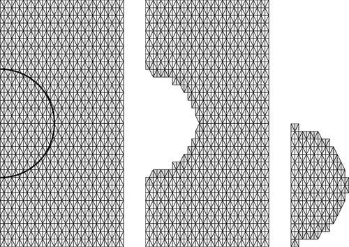
 . If the interface coincides exactly with an element edge, no new basis functions are introduced on these elements, but the approximating functions may still be discontinuous over such an edge. As a consequence, there are six non-zero basis functions on each element that properly intersects Γ. Perhaps this process is most easily seen as creating two new separate meshes with doubling of the elements crossed by the interface (Figure 1).

 to the order h in the norm
 . For this purpose, we construct an interpolant of v by nodal interpolants of H2-extensions of v1 and v2 as follows. Choose extension operators Ei:H2(Ωi)→H2(Ω) such that
 and
and
 (9)
(9) (10)
(10) be an interpolation operator defined as in 10. Then
 (11)
(11) (12)
(12)The crucial fact is that the constant in this inequality is independent of the location of the interface relative to the mesh. Optimal interpolation estimates follow, as does optimal convergence of the method irrespective of the location of the interface relative to the mesh. The key elements of the analysis are the robust coercivity of ah(·,·) with respect to the norm
 , the consistency property 8, and the approximability 11. For details, see 5.
2.2 The case of Dirichlet boundaries
 (13)
(13) that contains Ω but is not fitted to the domain boundary. Denoting the mesh domain
 , we consider the following finite element space:

 , we denote the set of elements that are intersected by the interface. For an element
 , let ΓK:=Γ∩K be the part of Γ in K. We also introduce the set of element faces
 associated with
 , defined as follows: for each face
 , there exist two simplices K and K′ such that F = K ∩ K′ and at least one of the two is a member of
 . This means in particular that the boundary faces of the mesh
 are excluded from
 . On a face F such that F = K ∩ K′, define the jump of the gradient of v∈Wh by
 , where nF denotes the unit normal to F, the orientation is chosen arbitrarily. The problem that arises when applying Nitsche's method in this framework is that the inverse inequality corresponding to 12 cannot be robust when the right hand side must be controlled by norms over the physical domain alone, as the cut elements can be arbitrarily small. We thus need to further stabilize the problem. The finite element discretization takes the form: find U∈Wh, such that
 (14)
(14)

 (15)
(15) (16)
(16) . Details are given in Section 3.
2.3 Other interface conditions of interest
- Heat release at the interface leads to
where g is a heat source term. This source leads to a modified right-hand side in 8 so that
 (17)see 5.
- Spring-type boundary conditions common in solid mechanics can be modeled by
Here, k denotes the compliance of distributed springs on the interface. These conditions can be modeled by Nitsche's approach as follows. Let sh=1/(h/γ + k)and modify the bilinear form to
 (18)The analysis of this method follows the same lines as the one for the original method; cf. 7, 23.
- Transport also on the interface can be modeled by
where ∇Γ is the tangential derivative on Γ,
 (19)These conditions model, for example, porous media flow in a medium with a crack represented by Γ; cf. 24. Here, αΓ represents a porosity along the crack. The bilinear form must now be modified to take the differential equation on Γ into account: formally replacing g in 17 by ∇Γ·(αΓ∇Γu), we see that a consistent bilinear form is given by
 where {a}:=k2a1+k1a2, with k1 and k2 positive weights. This method requires additional stabilization in general; cf. the numerical example in Section 6.4.
-
Alternative surface transport conditions are given by seeking u:Ω→R and uΓ:Γ→R, where Γ denotes the boundary of Ω, such that
Here, uΓ is a concentration on the surface, which is independent of the concentration inside Ω. Applications are found, for example, in cell membrane transport; cf. 25. Here, we no longer have a distinct side condition and can dispense with Nitsche's method. However, with cut elements, we now need a way to define the discrete approximation of uΓ, which is different from the previous case, where the trace spaces on the cut elements were used to compute ∇ΓU. An obvious idea is to keep on using the trace spaces on a higher dimensional mesh as suggested by Olshanskii et al. 26. Thus, we let (20)
(20) denote the space of continuous piecewise linear polynomials defined on
 and seek U∈Wh and
 such that
and
 (21)or the symmetrized version
 (22)
(22) (23)
(23)for all
 . The discretization of the equation on the interface can now be stabilized by adding
related to the stabilization in the Dirichlet case but with another scaling because of dimensionality. The bulk variable can be stabilized as in the Dirichlet case.
3 Enhancing Robustness: Ghost Penalty
Cutting the mesh can result in boundary elements with very small intersections with the physical domain, or for PDEs on embedded surfaces, bulk elements with very small intersection with the surface domain. This may lead to a poorly conditioned system matrix or failure of stability of the discrete scheme.
Situations that are particularly sensitive are the imposition of Dirichlet boundary conditions 12, 27, or domain decomposition on unfitted meshes, where an inf-sup condition has to be satisfied, such as for incompressible elasticity 9, 28-31. In these cases, one cannot choose the weights in 3 in a robust way. There are also situations where the weights are already prescribed by other concerns. This is the case in fluid–structure interaction 32, 33, where the elastodynamic system has no dissipation by which one can absorb the contribution of the boundary stress term and therefore only the fluid stresses are considered on the boundary. If independent adaptive mesh refinement is performed in the two subdomains of 5, this also imposes a certain choice of weights to ensure robustness, both with respect to large contrast in the physical parameter and in the mesh parameter 34.
For cases such as this, a useful trick 12, 27 is to add a penalty term in the interface zone that extends the coercivity to the whole mesh domain, that is, in the O(h) zone of the mesh domain of each subdomain that does not intersect the associated physical domain. This penalty term must be carefully designed to add sufficient stability, while remaining weakly consistent for smooth solutions. To illustrate this idea, we consider the fictitious domain method for the Poisson problem 13 with α = 1. In the next section, we demonstrate how these arguments can be extended to the coupled problem 1 and how the two formulations are related.

 (24)
(24)
 and
and
 . It follows that in principle we obtain coercivity by choosing
 , since by an arithmetic–geometric inequality, we have

 , the volume measure
 can be arbitrarily small.
 . Indeed, one may show the following inequality:
 (25)
(25) (26)
(26) (27)
(27) , where the lower bound is independent of the mesh/boundary intersection, but not of the penalty parameter γ1 in j(·,·). Error estimates now follow in a similar fashion as for the standard Nitsche's method, using 27 and 26. Indeed, provided the solution is smooth enough, there holds

3.1 Example: perfect conductor, the limit of infinite diffusion
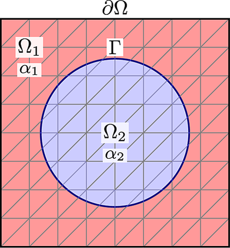
As an example of how the improved robustness works, we will consider the problem 1, with Ω2 completely enclosed by Ω1 such that ∂Ω⊂∂Ω1 and Γ:=∂Ω2(Figure 2). It is well known that in the limit α2→∞, the solution u2 becomes constant in Ω2 and can therefore be exactly represented by one degree of freedom. We will give two formulations of this problem, one similar to 5, and the other using the reduced model in a framework similar to the fictitious domain approach 14 using only one degree of freedom to represent u2. In both formulations, we will use the ghost penalty method so that the weights may be depending only on the diffusivities. This allows us to show that the solution of the domain decomposition approach converges to that of the fictitious domain approach in the limit as α2→∞. We will then compare this to what is obtained if the weights are chosen as in equation 4, with the penalty defined in equation 6 or 7.
 (28)
(28) (29)
(29) (30)
(30) . It is straightforward to prove coercivity of this formulation using the arguments of the previous section, indeed,
 (31)
(31)
 such that for all
 , there holds
 (32)
(32) . It follows by inspection that this formulation is equivalent to 14, with the only difference that in this case the Dirichlet value set on Γ is an unknown constant value. The coercivity and hence the discrete wellposedness can be shown here exactly using the arguments of 27 together with a triangle inequality and a trace inequality to get control of
 . First note that by a triangular inequality, a trace inequality on the whole domain Ω1, and a Poincaré inequality, we have

 (33)
(33) denote the solution of 32. If we set
 and note that
 , we may use the coercivity proven in 31:

 , we see that

 to write
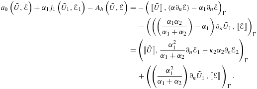 (34)
(34)

 as α2→∞ meaning that the asymptotic limit of the solution of 28 coincides with that of 32.
Another important observation is that for the discretization using ghost penalty and weights depending only on the diffusion, preconditioning the system matrix using diagonal scaling with α1,α2 leads to a system whose condition number is independent of both the mesh/boundary intersection and the contrast in the diffusion (for details, see 35).


3.2 A numerical illustration
Robustness issues may also appear in the limit of vanishing diffusion in a subdomain. We consider a configuration similar to that of Figure 2, with the square domain Ω:=[−1,1]2. Let Ω2 be a disc with radius 0.75 centered in the origin and Ω1:=Ω∖Ω2. In this configuration, we solve 1, with u|∂Ω=0, α1=1, f = 1,
 ,
,
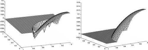
 and with α2∈{10−4,10−6,10−9}. First, we apply the formulation 5 with weights given by 3. The elevations of the solutions are presented in Figure 3. We then solve the same problem using the method 28 with 29–30 and give the corresponding elevations in Figure 4. Observe the relatively strong, but local, spurious overshoots that are present close to the layer in Figure 3. The combination of the ghost penalty and the parameters 29–30 eliminates the oscillations by relaxing the continuity constraint in the limit. Indeed, the sharp layer is represented as a discontinuity when it is under resolved.


Now, we consider the case where
 , α2=1 and choose α1=1020, to illustrate the effect in the limit α1→∞. This corresponds to a situation similar to that explored in Example 3.1, but with the diffusivity going to infinity in the outer domain. In Figure 5, we compare the results of the method 5 with the weights 3 and of 28 with 29–30. We see that for this large contrast, the method using the weights 3 exhibits some spurious oscillations close to the boundary, probably owing to an incompatibility between the constraint 〚U〛 = 0 and the weakly imposed condition on the gradient. In other words, the finite element space defined on the cut mesh does not allow for a H1-conforming interpolant that also can represent the jump in the gradient. This effect is reminiscent of locking but only present in the vicinity of the interface. The method 28 on the other hand converges to the fictitious domain solution of 14 in the limit for which optimal error estimates exist.
3.3 Ghost penalty for surface partial differential equations
 (35)
(35) such that
 (36)
(36) is the space of continuous piecewise linears on
 , the union of elements intersecting Γ.
 (37)
(37) (38)
(38) (39)
(39) (40)
(40) of v∈Wh and the L2-norm on
 , we may prove 37; see 38 for details.
 (41)
(41) (42)
(42)4 Discretizing Geometry in CutFEM
The starting point for the discretization of the geometry in CutFEM is to immerse an arbitrary geometric description in a background mesh. This mesh is typically chosen structured, to facilitate the handling of data structures, communication, and hierarchic mesh adaption. The discretization space and the variational formulation are then adapted to the geometry so that suitable boundary and interface conditions are imposed weakly as described in Section 2. This approach leads to some challenging implementation issues that we will describe later. It is advantageous to choose one particular geometry description that is versatile and simple for the construction of the discretization. Other geometrical descriptions can then be either included using modules that translate different formats to the one chosen to interface with the code or provided with their own CutFEM modules.
 . More precisely, a given domain
 can be decomposed into an inner part Ω1, an outer part
 , and their common interface Γ by requiring that ∀x∈Ω
 (43)
(43) as the (open) complement of Ω1 in Ω.
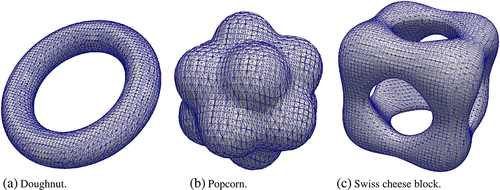
To give a few non-trivial examples of analytically given level-set based surface descriptions, we introduce
The corresponding surfaces are depicted in Figure 6.
Using a level-set description, complex domains can easily be constructed by translating Boolean set operations and geometric transformations into simple manipulations of level-set representations. For instance, given two level set functions φ1 and φ2 representing the domains Ω1 and Ω2, respectively, the level-set function representing the result of a standard Boolean set operation can be constructed according to the following table:
Moreover, for any diffeomorphic mapping
 , the mapped domain
 is represented by
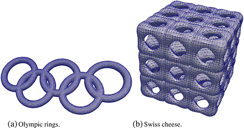
 . Figure 7 illustrates how complex surfaces can be generated by combining these operations.
5 Implementational Aspects of a Level-set Based CutFEM Method
We now briefly review some of the data structures and algorithms required to efficiently compute a discrete representation of surfaces implicitly given by a level-set and how to evaluate the variational formulation on this discrete geometry. An important step here is the introduction of a subtriangulation of cut elements to facilitate integration, which we will describe in more detail below. This subtriangulation is used only for integration so that the resulting subtriangles are not constrained by the conformity requirements of the finite element space. In addition, their aspect ratio does not impact the approximation properties of the discretization, because they are never used in the analysis.
In general, the mesh subdivision can be characterized as follows. Referring to the notation from Section 2, we recall that for a tessellation
 of Ω, the (unfitted) surface Γ leads to natural subdivision
 , where
 . Note that, to apply the finite element method to a pure surface problem, we only need to compute a tessellation of Γ with respect to
 . For a fictitious domain problem, we require a subtesselation for the inner part of the cut elements
 and for an interface problem, we need to subtriangulate both the inner and outer parts, that is, also
 . However, as the following section will explain, all these sub-triangulations can be provided simultaneously by using the well-known marching tetrahedra algorithm 39, 41.
In addition to this subtesselation algorithm, routines for the computation of integrals over cut cell parts have to be provided. Indeed, for each intersected element
 , volume integrals have to be evaluated over the parts of K that are covered by the two physical subdomains Ω1, K1=K∩Ω1 and Ω2, K2=K∩Ω2. To construct the matrix contributions that impose interface and boundary conditions, surface integrals over interface segments, ΓK=Γ∩K, that lie within the element
 , also have to be computed.
In the following, we will first detail our implementation of the classical tetrahedra algorithm 39, 41 and then give some further details on how to evaluate integrals over cell parts.
5.1 Interface approximation and sub-triangulation of cut elements
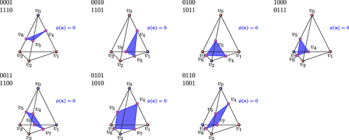
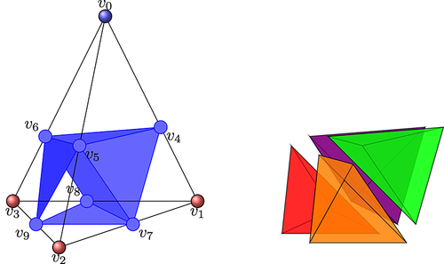
In the first step of the subtesselation algorithm, the values of the level-set function in the element nodes are used to distinguish between elements that are fully contained in Ω1 (φ < 0 for all nodes) or Ω2 (φ > 0 for all nodes) and the elements that are intersected by the interface Γ (φ > 0 and φ < 0 in some nodes) (Figures 8 and 9).

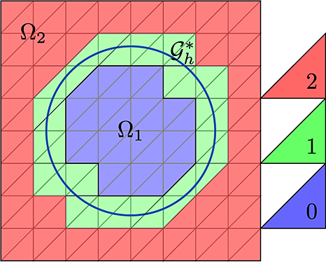
For elements that are intersected by the interface, we perform a subtriangulation of the element allowing us to apply standard quadrature rules to the subtriangles for the integration over the parts K1, K2, and ΓK. Here, we only consider linear intersections of the zero level-set with the elements that are represented by one straight line segment per element in 2d or one plane in 3d. In more detail, the subtriangulation algorithm consists of the following steps.
- Flag cells according to which nodes of the element have a negative level-set value (flag with ‘1’) and which nodes have a positive level-set value (flag with ‘0’).
- Use this flag in order to compute the intersection points of the zero level-set with element facets via linear interpolation between the level set values in the nodes connected to the facet. Note that an intersected facet is characterized by the fact that the values of the level-set function in the nodes connected to that facet have positive and negative values of the level-set function.
-
Build a subtriangulation of each cut cell part, that is, K1, K2 and ΓK. The subtriangulation of Ki, i = 1,2, and the sub-triangulation for ΓK are then added to the subtesselation for the inner part of the cut elements
 , the outer part of the cut elements
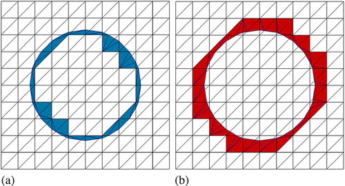
 , or the tessellation of Γ, respectively (Figure 11), together with a map between the cell parts and the corresponding parent cell.
In two space dimensions, the cut cell parts, K1 and K2, are either triangular or quadrilateral (Figure 10). The triangular part can be added directly to the subtriangulation of the corresponding domain. The quadrilateral part is subdivided into two triangles first and then added to the corresponding subtriangulation. The interface segment ΓK is represented by straight line segment connecting both intersection points. These interface line segments are stored in a separate mesh object with topological dimension 1. The resulting sub-triangulations for Ω1 and Ω2 for a circular domain Ω1 are shown in Figure 11.
In three space dimensions, there is a much wider range of cut cases to consider. We can distinguish 14 cases, among which eight have a triangular interface plane cut of the zero level set with the tetrahedron and six with a quadrilateral interface plane cut (Figure 12). The triangular plane cut can be added directly to the subtriangulation of the two-dimensional zero level set interface representation, and the quadrilateral planes are subdivided into two triangular parts. For the volume subtriangulation, we decompose the tetrahedron into eight subtetrahedra (Figure 13) and add the subtetrahedra to the corresponding subtesselations of Ω1 and Ω2 depending on the cell flag, that is, depending on whether they lie in Ω1 or Ω2.

5.2 Integration over subtriangulation
For the evaluation of integrals over the subtriangulation, we require two mappings
 . Here, the linear affine mapping, χp, between the reference element and the cell part, transforms a quadrature rule defined on the reference element in terms of quadrature points ξi and weights wi into a quadrature rule on the subtriangle cell part (Figure 14). The mapping χw between the reference element and the whole ‘parent’ cell is used to map the quadrature points defined on the physical subtriangle to their location in the reference element of the whole parent cell.
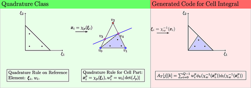
 and quadrature weights
 . Here, Jp is the Jacobian of the mapping χp. These points and weights can then be used to perform the numerical quadrature over the given cell part, for example, for a mass matrix, by
 (47)
(47) that result from the backward transformation of the quadrature rule over the cell part onto the reference element of the whole ‘parent’ element.
5.3 Software for CutFEM-type method
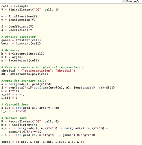
The technology required for the automated assembly of general cut finite element based variational forms over fictitious domains and embedded surfaces has been implemented as part of the software library libCutFEM. libCutFEM is open source and freely available from http://www.cutfem.org. This software library builds on the finite element library DOLFIN, which is part of the FEniCS project 42 for automated scientific computing. The main feature of FEniCS is the automated treatment of finite element variational problems, based on automated generation of highly efficient C++ code from abstract high-level descriptions of finite element variational problems expressed in near-mathematical notation 43.
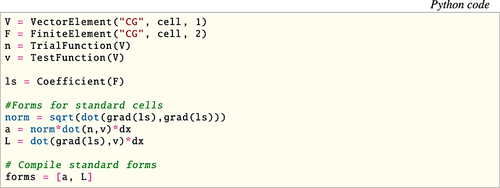
libCutFEM makes use of this automatization technology in the following way. We specify the variational problem in near-mathematical notation in the domain specific Uniform Form Language 43 (for an example, see Figure 17). Then the code generation components of FEniCS (UFL+FFC+UFC 42) generate code containing information about the cell integrals of the given forms and information about the elements such as the degrees of freedom maps. In particular, libCutFEM uses an extension developed in earlier works of the components FFC 44, 45 and UFC 46. In these works, FFC and UFC were extended 33, 47, 48 to provide generated code for the cell integration over cut cell parts (see right box in Figure 14). These extensions provide the fundamental infrastructure for the evaluation of cut finite element based variational forms defined on fictitious domains and embedded surfaces. Consequently, given a high-level description of the variational formulation, low-level C++ code can be automatically generated for the evaluation of the cut element and surface integrals, in addition to the evaluation of integrals over the standard (non-cut) mesh entities. The generated code takes as input appropriate quadrature points and weights for each cut entity, which are provided by the libCutFEM library. The resulting cell integral matrix contributions are then assembled to the global matrix by routines provided in libCutFEM.
In addition to these quadrature and assembly routines, libCutFEM provides functionality for computing topological and geometric descriptions of the embedded surface and cut elements. Currently, libCutFEM mainly supports the level set based cutting algorithm as described in detail in the previous section. However, alternative geometrical algorithms can be integrated easily thanks to the modular structure of the library and FEniCS, which decouples the variational formulation, the quadrature and assembly routines, and the geometrical and mesh description.
In summary, in libCutFEM, one may specify variational forms defined over finite element spaces on fictitious domains in high-level UFL notation 43, define the background mesh
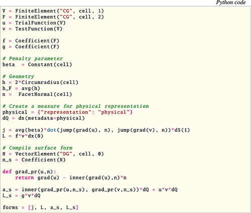
 , and give a description of the surface Γ, and then invoke the functionality provided by the libCutFEM library to automatically assemble the corresponding stiffness matrix. In particular, the numerical experiments presented in Sections 6.1–6.3, corresponding to the variational formulation defined by 50, 58 and 60, have been carried out using this technology. We also present the UFL scripts that were used to obtain the numerical results illustrating the simplicity by which the end user can access the CutFEM paradigm (Figures 17, 18, and 21). Other software projects including CutFEM style technology include GetFem++ 49, LifeV 50, and DUNE-UDG 51.
6 Numerical Results
6.1 Stabilized Nitsche fictitious domain method for the Poisson problem
 (48)
(48) (49)
(49) (50)
(50) (51)
(51) (52)
(52) (53)
(53) (54)
(54) (55)
(55) such that
 (56)
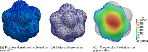
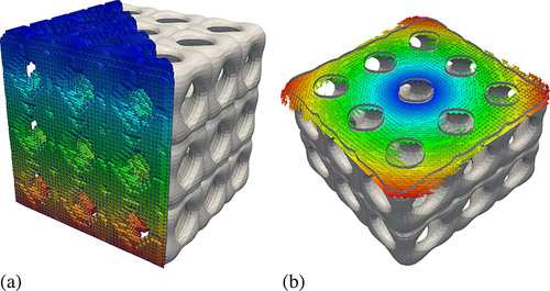
(56)The solution u in the popcorn geometry is depicted in Figure 15. Figure 15a shows the fictitious domain mesh of the popcorn geometry colored by the value of U. Figure 15b displays the subtesselation of the popcorn surface, and Figure 15c shows a contour plot of U in a slice through the middle of the popcorn.
Solving the Poisson Equation 50 in the olympic ring geometry gives the result depicted in Figure 16, where Figure 16a shows the surface subtesselation, and Figure 16b shows the solution U in a slice through the middle of the olympic rings. The UFL input files to specify Equations (50 and 56 in the libCutFEM/FEniCS framework are displayed in Figures 17 and 18, respectively.

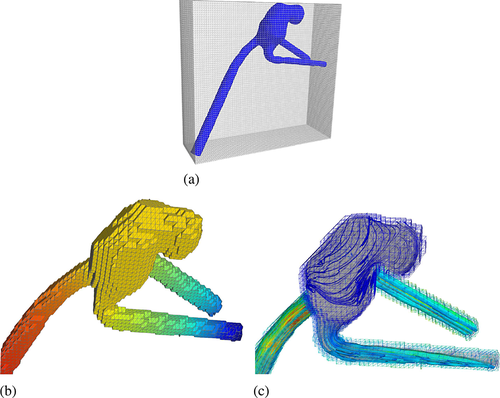
6.2 Stabilized Nitsche fictitious domain method for the Stokes' problem

 -vector fields and let the discrete pressure space Qh consist of either piecewise constant or continuous piecewise linear elements, denoted by
 and
and
 , respectively. To formulate our CutFEM method for the Stokes problem, we introduce the forms


 and
and
 are known to violate the Babuška–Brezzi conditions, we stabilize our scheme by the following symmetric pressure penalties:
 (57)
(57) denotes all the interior faces in the mesh domain
 . Note that the integral contributions in 57 are always evaluated on the entire face F, even for faces that are intersected by the boundary Γ. Again, such a ghost penalty ensures the robustness and optimal convergence properties of the stabilized scheme irrespective of the location of the boundary; see 29, 30 for detailed proofs.
 (58)
(58)

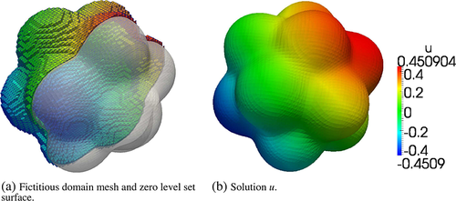
6.3 Laplace–Beltrami problem on a surface using a bulk-mesh
 solving
 (59)
(59) such that
 (60)
(60) (61)
(61) (62)
(62)
6.4 Porous media flow in a domain with cracks

We consider the following model problem in
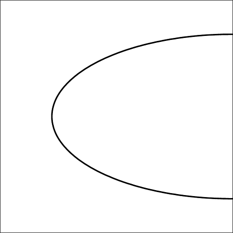
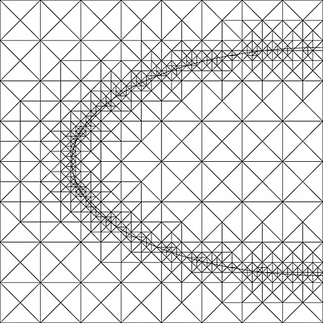
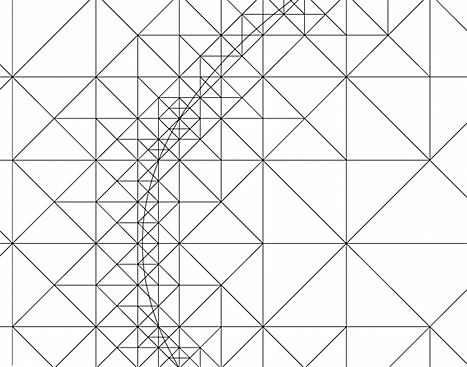
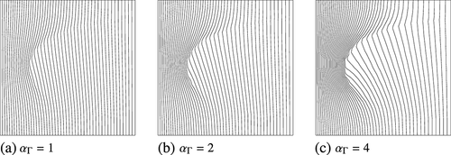
 : a domain (0,1) × (0,1) with Dirichlet boundary conditions u = 1 at x = 0 and u = 0 at x = 1, zero Neumann conditions elsewhere. Choosing α = 1 in Ω and an elliptically shaped crack shown in Figure 23 and setting γΓ=10, we obtain the following results when setting αΓ=0 on the lower arc of the crack and αΓ∈{1,2,4} in the upper arc. A close-up of the computed velocities α∇U close to the crack, using the computational mesh of Figure 24, is shown in Figure 25, together with a corresponding zoom of the mesh in Figure 26, and isoline plots of the pressures U are given in Figure 27. We note that even a small increase in permeability increases the velocity quite noticeably in the crack. Further developments for system of cracks are under way.

7 Concluding Remarks
In this paper, we have given an exposition of recent results on CutFEM combined with Nitsche's method and ghost penalty stabilization. The main theoretical ideas have been discussed, but emphasis has been put on implementation issues in the setting of the FEniCS software project.
We have endeavored to show the versatility of the CutFEM method as a method for fictitious domain computations, overlapping mesh methods, multiphysics coupling between a bulk domain and its surfaces or embedded interfaces, and model coupling problems. In particular, we have pointed out the possibility of posing and solving PDEs on interfaces/surfaces as well as in the bulk.
In conclusion, the results reported here (and in the references) show that CutFEM holds great promise as a versatile and powerful mesh-free method posed on a mesh. Challenges currently being investigated include optimization techniques using surface sensitivities, and moving interfaces, for example, for free surface problems.
Acknowledgements
This research was supported in part by EPSRC (first and second authors, Grant No. EP/J002312/2), in part by the Swedish Foundation for Strategic Research (second and third author, Grant No. AM13-0029) and the Swedish Research Council (second and third author, Grants No. 2011-4992 (PH) and No. 2013-4708 (MGL)). The work for this article was also supported by a Center of Excellence grant from the Research Council of Norway to the Center for Biomedical Computing at Simula Research Laboratory.


