Adapting standardized trout monitoring to a changing climate for the upper Yellowstone River, Montana, USA
Abstract
Objective
Long-term standardized monitoring programs are fundamental to assessing how fish populations respond to anthropogenic stressors. Standardized monitoring programs may need to adopt new methods to adapt to rapid environmental changes that are associated with a changing climate. In the upper Yellowstone River, Montana, biologists have used a standardized, mark–recapture monitoring protocol to annually estimate the abundance of trout since 1978 to assess population status and trends. However, within the past two decades, climate change has caused changes in discharge timing that have prevented standardized monitoring from occurring annually.
Methods
We investigated the feasibility of using two analytical methods, N-mixture models and mean capture probability, for estimating the abundance of three trout species in the upper Yellowstone River using the historical long-term data set; these methods allow abundance to be estimated when a mark–recapture estimate cannot be obtained due to hydrologic conditions.
Result
When compared with abundance estimates from mark–recapture methods, N-mixture models most often resulted in negatively biased abundance estimates, whereas mean capture probability analyses resulted in positively biased abundance estimates. Additionally, N-mixture models produced negatively biased estimates when tested against true abundance values from simulated data sets. The bias in the N-mixture model estimates was caused by poor model fit and variation in capture probability. The bias in the mean capture probability estimates was caused by heterogeneity in capture probability, likely caused by variable environmental conditions, which were not accounted for in the models.
Conclusion
N-mixture models and mean capture probability are not viable alternatives for estimating abundance in the upper Yellowstone River. Thus, exploring additional adaptations to sampling methodologies and analytical approaches, including models that require individually marked fish, will be valuable for this system. Climate change will undoubtedly necessitate changes to standardized sampling methods throughout the world; thus, developing alternative sampling and analytical methods will be important for maintaining the utility of long-term data sets.
INTRODUCTION
Long-term standardized monitoring programs are fundamental for assessing how fish populations respond to anthropogenic stressors and changing environmental conditions (Radinger et al. 2019). Standardized monitoring data are commonly used to measure changes in the abundance and distribution of fishes over space and time and provide valuable information for management decisions, especially in an adaptive management context (Schreiber et al. 2004; Bonar et al. 2009; McClelland et al. 2012; Wagner et al. 2013; Hansen et al. 2015). Long-term monitoring requires standardization to identify trends and make temporal comparisons; however, monitoring may be adapted as technology, questions of interest, and the sampling feasibility change (Lindenmayer and Likens 2009). Adapting existing monitoring programs will likely become increasingly important as climate change alters environmental conditions (Lindenmayer and Likens 2009; Lindenmayer et al. 2011). Adaptive monitoring may include developing and implementing new monitoring protocols, adjusting the frequency of sampling, addressing new questions and hypotheses related to climate change, and adopting new analytical methods (Paukert et al. 2016; Shirk et al. 2023).
In the upper Yellowstone River, Montana Fish, Wildlife and Parks (MFWP) biologists have been monitoring the abundance of nonnative Rainbow Trout Oncorhynchus mykiss, Brown Trout Salmo trutta, and native Yellowstone Cutthroat Trout Oncorhynchus virginalis bouvieri since 1978. The monitoring program consists of annual mark–recapture surveys to estimate the abundance of the three trout species, which support a valuable recreational fishery that contributed an estimated US$70 million to the local economy in 2013 (Sage 2016). Mark–recapture surveys consist of a marking survey and a recapture survey, and Lincoln–Petersen mark–recapture methods are used to estimate trout abundance. In southwestern Montana, climate change is altering the timing and duration of spring snowmelt runoff (Hostetler et al. 2021), and these changes have prevented trout monitoring from occurring consistently in the upper Yellowstone River over the past two decades. Specifically, warming spring temperatures cause the river discharge to increase from baseflow conditions to peak runoff conditions more quickly (Figure S1 available in the Supplemental Material in the online version of this article), resulting in a reduced period when sampling can occur because of the reduced capture efficiency at high discharge (Lamborn and Smith 2019). A reduced sampling period has prevented a recapture survey from occurring in some years and has occasionally prevented all sampling from occurring, and abundance estimates cannot be obtained in these years. Thus, changes in discharge patterns have resulted in numerous gaps in the annual abundance data for the monitored species, making it difficult to identify trends in population abundance (Opitz 2021). Gaps in monitoring data are of particular concern for the endemic Yellowstone Cutthroat Trout, which are a focus of conservation efforts throughout the upper Yellowstone River watershed (Endicott et al. 2013). Thus, the standardized monitoring program for the Yellowstone River must be adapted to continue the long-term monitoring program in a changing climate.
Novel methods for estimating the abundance of animal populations have been developed in recent years, giving biologists more flexibility when designing and implementing monitoring programs (Williams et al. 2002; Kéry and Royle 2015). Here, we explore two analytical methods, N-mixture models and mean capture probability, as alternatives to the Lincoln–Peterson mark–recapture methods that historically have been used for the Yellowstone River trout populations and other trout populations across Montana. N-mixture models use replicated count data from unmarked animals to estimate abundance and capture probability (Royle 2004). N-mixture models have commonly been used with mammals, birds, and herpetofauna (McCaffery et al. 2016; Williams et al. 2017; Ficetola et al. 2018) but are less commonly applied to fish populations (but see Som et al. 2018; Vine et al. 2019). We used N-mixture models to estimate both abundance and capture probability from the number of sampled fish during electrofishing surveys. In addition to N-mixture models, we took advantage of long-term data on capture probability from the mark–recapture estimates to estimate abundance, using capture probability as either a mean or a running average. Both the N-mixture models and mean capture probability use the current long-term data set, allowing us to maintain continuity, which is an important component of adaptive monitoring (Lindenmayer and Likens 2009). Additionally, both methods can be used to estimate abundance from a single sample per year (Mitro and Zale 2000; Costa et al. 2019).
We investigated the feasibility of using N-mixture models and mean capture probability to estimate abundance of three trout species in the upper Yellowstone River using the existing, long-term data set spanning 44 years, from 1978 to 2021. Our research objectives for each trout species were (1) to compare abundance estimates from N-mixture models and Lincoln–Petersen mark–recapture models to determine whether N-mixture models provide a viable alternative method for estimating trout abundance, (2) to evaluate whether estimates from N-mixture models are biased relative to abundance values from simulated data sets, and (3) to compare mean capture probability and Lincoln–Petersen mark–recapture abundance estimates to determine whether mean capture probability methods can be used as an alternative method for estimating trout abundance. This research improves our understanding of the utility of two analytical methods for long-term standardized monitoring programs under increasingly challenging environmental conditions.
METHODS
Study area
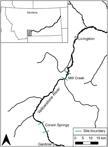
The Yellowstone River originates in the Bridger-Teton National Forest in northwestern Wyoming and flows 1114 km to the confluence with the Missouri River in western North Dakota (Figure 1). It is the longest unregulated river in the contiguous United States. The hydrologic regime of the Yellowstone River is snowmelt driven, with a large peak in discharge in the late spring during runoff. Our study area consists of two long-term sampling sites, Corwin Springs and Mill Creek, located between Gardiner and Livingston, Montana (Figure 1). The boundaries of the sampling sites have varied slightly among years; the mean length of the Corwin Springs site is 7.66 km (standard deviation (SD) = 1.52 km), and mean length of the Mill Creek site is 7.60 km (SD = 0.85 km).
Mark–recapture
Mark–recapture sampling was conducted by MFWP biologists beginning in 1978 at Corwin Springs and 1980 at Mill Creek annually during a period of 1–2 weeks at each site, when local populations could reasonably be assumed to be closed to changes in size due to births, immigration, deaths, or emigration (Otis et al. 1978). Historically, monitoring was conducted in mid-April to early May when the discharge of the Yellowstone River was favorable for electrofishing, between 56 and 142 m3/s (horizontal dashed lines in Figure S1). Electrofishing was most often conducted using one or two outboard jet boats mounted with boom electrofishing equipment; however, drift boats or rafts were used for sampling from 2008 to 2010 at the Corwin Springs site due to variable discharge conditions. The boats were each equipped with a Smith Root VVP-15B and a Honda generator (Opitz 2021) and had one or two netters. Output amperage was standardized between 2.5 and 3.0. Each survey consisted of electrofishing along both riverbanks. When two jet boats were available, the two boats would electrofish along the left and right banks simultaneously; when one boat was used, electrofishing along each bank occurred separately over 1 or 2 days. Each fish was identified to species and measured to the nearest 2.5 mm (0.1 inches) following MFWP standard protocol. During the marking sample, each fish was marked with a pelvic fin clip and released at the site where it was sampled. A recapture sample occurred about 7 days after the marking sample, allowing the marked fish to mix with the population. Both marking and recapture samples were conducted in 32 out of 44 years for the Corwin Springs site. In four additional years, a marking sample was conducted but flow conditions prevented the recapture sample from occurring, resulting in data from a single electrofishing survey only; in the remaining 4 years, no sampling occurred. For the Mill Creek site, both marking and recapture samples were conducted in 33 out of 42 years and a marking sample only was conducted in two additional years. In the remaining 5 years, no sampling occurred.
Statistical analysis
Mark–recapture
We used a Chapman-modified Lincoln–Petersen estimator to estimate the population size of Yellowstone Cutthroat Trout, Rainbow Trout, and Brown Trout ≥178 mm in total length at each site. The estimates were divided by the length of the site to estimate the number of fish per kilometer each year. Chapman-modified Lincoln–Petersen mark–recapture abundance estimates (hereafter, “mark–recapture estimates”) were only calculated for years when both marking and recapture surveys were conducted. All the analyses were conducted in R version 4.3.1 (R Core Team 2023). The mark–recapture estimates were calculated using the mrClosed() function in the FSA package in R (Ogle et al. 2023).
N-mixture models
We used N-mixture models to estimate the abundance of each trout species at Corwin Springs from 1978 to 2021 and Mill Creek from 1980 to 2021. A time-for-space substitution approach was used; therefore, we modeled each site and species separately (Costa et al. 2019, 2021). The number of fish that was sampled during each survey was used as count data. The mark and recapture surveys served as replicate site visits, so our data set included up to two site visits per year. Using a time-for-space substitution approach allowed us to estimate abundance in years with only a single site visit (Costa et al. 2019). We fit three N-mixture models for each site and species combination: a Poisson N-mixture model with no covariates, a negative binomial N-mixture model with no covariates, and a Poisson N-mixture model with river discharge included as a covariate to model capture probability. We did not consider a negative binomial N-mixture model with river discharge due to unstable estimates from the negative binomial N-mixture model with no covariates. Discharge data were obtained from the U.S. Geological Survey stream gauge at Corwin Springs, Montana, located at the southern boundary of the Corwin Springs sampling site (U.S. Geological Survey 2023). Mean daily discharge on each day when sampling was conducted was used as a covariate for capture probability.
When fitting the Poisson N-mixture models, the upper limit of integration, K, was set to 2000; this value was selected because it was higher than the largest observed count for any site or species and increasing the value of K above 2000 did not affect the estimates (Kéry and Royle 2015). Models were considered unstable if the estimates continually increased as values of K increased. Abundance was estimated for trout species in each year from the posterior distribution of the latent abundance using the ranef() function from the unmarked package, and all N-mixture models were fit using the pcount() function in the unmarked package in R (Fiske and Chandler 2011). The model fit of the N-mixture models was assessed using the nmixgof package in R (Knape et al. 2018). We assessed overdispersion, using the overdispersion parameter ( = 1 indicates no overdispersion) and examined quantile–quantile plots of randomized quantile residuals for normality (Knape et al. 2018). To compare the abundance estimates from the N-mixture models with the mark–recapture estimates, we calculated relative bias as the difference between the N-mixture abundance estimate and the mark–recapture abundance estimate divided by the mark–recapture abundance estimate for each year. The median value of relative bias indicates whether the abundance estimates show consistent negative or positive bias relative to the mark–recapture estimates, whereas the spread of relative bias is used to assess the range of bias in estimates.
N-mixture modeling of simulated data sets
Simulations were used to assess the performance of the N-mixture models using empirical estimates of abundance and capture probability from the Yellowstone River. All abundance estimation methods may be biased, so the mark–recapture estimates may not represent the true abundance of trout in the upper Yellowstone River. The use of simulated data sets allowed us to compare the N-mixture model estimates with known abundance values. We then analyzed each data set and compared the abundance estimates from the N-mixture models with the simulated abundance values to evaluate the performance of models. To simulate the data sets, we used the simNmix() function from the AHMbook package in R (Kéry et al. 2022). The mean abundance and capture probability values from the mark–recapture estimates for each species and site were used as the mean abundance and capture probability values for the simulated data sets. Abundance was simulated using a negative binomial distribution, and values of capture probability were allowed to vary by sampling event to best approximate our observed data sets. Variation in capture probability was incorporated as a random effect on the logit scale that was obtained from a normal distribution with a mean of zero and a standard deviation of 0.3 (Kéry and Royle 2015). We simulated 500 30-year data sets for each site and species and fit Poisson N-mixture models to each data set. Each data set was simulated using two sampling events per year. To assess model performance, relative bias was calculated as the difference between the estimated and simulated values for abundance.
Mean capture probability
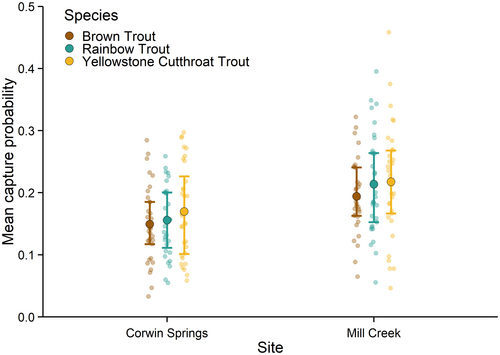
Mean capture probability was calculated from the long-term monitoring data set for each combination of species and site by averaging the capture probability point estimates from all years when mark–recapture estimates were completed (Figure 2) using the equation , where is the estimated abundance; is catch, defined as the number of fish captured during a marking electrofishing survey; and is estimated capture probability. We standardized the abundance estimates by reach length to estimate the number of fish per kilometer in each year. The variation associated with the estimate was obtained by dividing the number of fish that was sampled during the marking run by the 25th quantile of capture probability (upper limit) and the 75th quantile of capture probability (lower limit). A moving-average approach was used to account for the variation in capture probability over time. We calculated a 3-year moving average of capture probability; a 2-year moving average was used for the first and last years in the data set to avoid missing values. To estimate abundance, we divided the number of fish that we caught during the marking run by the moving average of capture probability for the appropriate year. The variation that was associated with the estimate was calculated as the number of fish that was caught during the marking run divided by the minimum capture probability from the 3-year window (upper limit) and the maximum capture probability from the 3-year window (lower limit). To compare the mean capture probability estimates with the mark–recapture estimates, relative bias was calculated using the same approach as was used for the N-mixture models.
RESULTS
Mark–recapture estimates
The mean number of sampled fish in each electrofishing survey varied from 144 (SD = 85) for Yellowstone Cutthroat Trout at Mill Creek to 450 (SD = 305) for Brown Trout at Mill Creek. The mark–recapture abundance estimates varied over time by species and site. Mean abundance over the entire study period was highest for Brown Trout at Mill Creek at 200 fish/km (SD = 116) and lowest for Yellowstone Cutthroat Trout at Mill Creek at 72 fish/km (SD = 52). The empirical estimates of mean capture probability varied from 0.15 to 0.22 for all sites and species (Figure 2).
N-mixture model fit
The N-mixture models resulted in unsatisfactory model fit for the data sets. Goodness-of-fit testing indicated that the data sets for each species and site displayed overdispersion, which resulted in poor model fit when using the Poisson N-mixture models. The overdispersion parameters () were >45 for all models, indicating strong overdispersion (Table 1). Additionally, an inspection of quantile–quantile plots indicated that the randomized-quantile residuals were not normally distributed (Figure S2). Including discharge as a covariate to model capture probability did not improve the model fit (Table 1). The negative binomial N-mixture models showed better model fit than did the Poisson N-mixture models. The values of were <3.5 for all models, and the randomized-quantile residuals were normally distributed (Table 1; Figure S2). However, the negative binomial N-mixture models resulted in unstable abundance estimates. Thus, the benefit of the improved model fit with the negative binomial N-mixture models is negated by the instability of the model, which prevented us from obtaining abundance estimates using this model type. Despite the high overdispersion, we moved forward with estimating abundance, using the Poisson N-mixture models to illustrate how model fit influenced the estimates of abundance and capture probability relative to the mark–recapture estimates and simulated data sets.
| Species | Site | Poisson | Poisson with discharge | Negative binomial |
|---|---|---|---|---|
| Yellowstone Cutthroat Trout | Corwin Springs | 45.18 | 93.76 | 1.68 |
| Mill Creek | 52.64 | 1892.60 | 1.81 | |
| Rainbow Trout | Corwin Springs | 79.73 | 94.13 | 1.57 |
| Mill Creek | 90.33 | 92.45 | 1.73 | |
| Brown Trout | Corwin Springs | 115.71 | 140.05 | 2.11 |
| Mill Creek | 226.77 | 253.94 | 3.35 |
Poisson N-mixture models
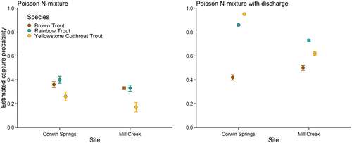
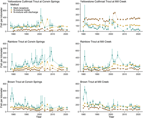
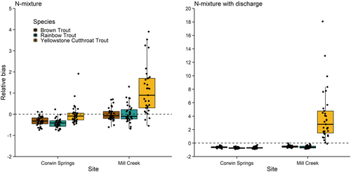
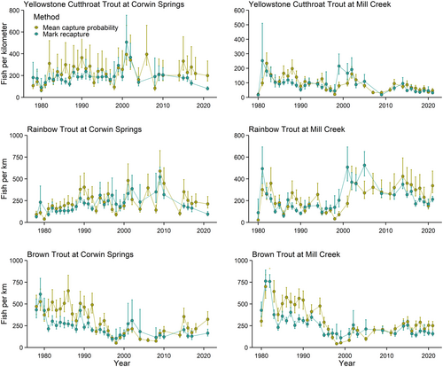
The Poisson N-mixture models produced estimates that were biased relative to the mark–recapture estimates. The estimated capture probabilities from the Poisson N-mixture models varied from 0.17 for Yellowstone Cutthroat Trout at Mill Creek to 0.40 for Rainbow Trout at Corwin Springs (Figure 3). The Poisson N-mixture models resulted in capture probabilities that were higher than the mark–recapture estimates for all sites and species except for Yellowstone Cutthroat Trout at Mill Creek (Figures 2 and 3). The N-mixture abundance estimates had lower interannual variation than the mark–recapture abundance estimates (Figure 4). The abundance estimates from the Poisson N-mixture models were generally lower than the mark–recapture abundance estimates, and therefore, median relative bias was less than zero for all sites and species, excluding Yellowstone Cutthroat Trout at Mill Creek (Figures 4 and 5). Relative bias was highest and had the largest spread for Yellowstone Cutthroat Trout at Mill Creek, with a median value of 1.20 and an interquartile range (IQR) of 1.46. (Figure 5).
Poisson N-mixture models with discharge
Mean daily discharge varied from 40 to 459 m3/s on the days when the surveys were conducted. The median value of daily average discharge was 80 m3/s when the surveys were conducted at Corwin Springs and 76 m3/s when surveys were conducted at Mill Creek. In general, including discharge as a covariate resulted in higher and unrealistic estimates of capture probability and lower estimates of abundance than were observed with the Poisson N-mixture models without a covariate (Figures 3 and 4). Median relative bias was below zero for all sites and species except Yellowstone Cutthroat Trout at Mill Creek, which had a median relative bias of 2.79 (Figure 5). The IQR was less than zero for all sites and species except for Yellowstone Cutthroat Trout at Mill Creek. Including discharge in the model resulted in higher discrepancy between the N-mixture model abundance estimates and mark–recapture abundance estimates (Figure 5).
N-mixture model simulations
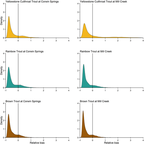
The Poisson N-mixture models generally underestimated abundance when they were fit to the simulated data sets using mean abundance and capture probability values from empirical data (Figures S3). The Poisson N-mixture models occasionally overestimated abundance for some simulated data sets but rarely resulted in accurate abundance estimates. Median relative bias was below zero for all sites and species (Figure 6).
Mean capture probability
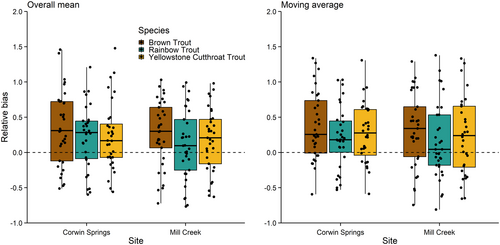
The abundance estimates from mean capture probability were generally higher than the mark–recapture estimates; however, there were instances where the mean capture probability estimates were lower than the mark–recapture estimates (Figure 7). Median relative bias was greater than zero for all sites and species (Figure 8). Median relative bias varied from 0.10 (IQR = 0.72) for Rainbow Trout at Mill Creek to 0.31 (IQR = 0.84) for Brown Trout at Corwin Springs. The IQR varied from 0.48 for Yellowstone Cutthroat Trout at Corwin Springs to 0.84 for Brown Trout at Corwin Springs. The spread of relative bias indicates the possibility of both over- and underestimating of abundance relative to mark–recapture abundance estimates. The median and IQR of relative bias were similar among all sites and species (Figure 8), indicating that the comparisons between the abundance estimates from mean capture probability and mark–recapture methods were similar by species and sites. The 3-year moving average of capture probability resulted in estimates that were comparable to the overall mean capture probability (Figure 8). Median relative bias when using the moving average of capture probability varied from 0.04 (IQR = 0.72) for Rainbow Trout at Mill Creek to 0.34 (IQR = 0.75) for Brown Trout at Mill Creek (Figure 8).
DISCUSSION
Identifying alternative methods for continuing standardized long-term monitoring of trout populations in the Yellowstone River is important as environmental conditions change. Our results indicate that neither N-mixture models nor mean capture probability analysis provided unbiased abundance estimates relative to the mark–recapture abundance estimates. Due to overdispersion and unmodeled heterogeneity in capture probability in our data set, the model fit of the N-mixture models was poor, resulting in unreliable estimates of abundance and capture probability. The N-mixture model estimates were most often lower than the mark–recapture estimates for all sites and species, excluding Yellowstone Cutthroat Trout at Mill Creek. Furthermore, the results of the simulations indicated that the estimates from the N-mixture models were biased relative to the true simulated abundance values. The mean capture probability analysis most often overestimated abundance relative to the mark–recapture abundance estimates. These results suggest that neither the N-mixture models nor the mean capture probability analysis are feasible alternatives to mark–recapture models for trout monitoring in the upper Yellowstone River. Thus, exploring other alternative sampling methods and analytical approaches will be needed for the study system.
Poor model fit due to limitations of the data set caused bias in the abundance estimates from the Poisson N-mixture models. Violations of parametric modeling assumptions can result in severe underestimation when abundance values are overdispersed (Knape et al. 2018), and the overdispersion parameters were high for all the Poisson N-mixture models in our analysis. To address the overdispersion in our data set, we fit negative binomial N-mixture models but were unable to obtain stable abundance estimates from these models. Negative binomial N-mixture models are more likely to result in unstable estimates or unidentifiable parameters, despite often showing better model fit than Poisson N-mixture models (Kéry and Royle 2015; Kéry 2018). Overdispersion also appeared to influence bias in the abundance estimates in our simulations. The N-mixture models generally underestimated abundance relative to the known simulated data sets, indicating that using N-mixture models to estimate abundance of trout in the Yellowstone River would result in biased abundance estimates. Reporting the estimates from the N-mixture models and proceeding with the simulation analysis despite indications of poor model fit provided a more complete understanding of how violations of model assumptions can affect resulting estimates and underscored the importance of assessing model fit, particularly when exploring new analytical approaches.
In addition to overdispersion, unmodeled heterogeneity in capture probability likely contributed to the bias in the N-mixture abundance estimates. Variation in capture probability is caused by numerous factors when electrofishing including environmental conditions, crew experience, electrofishing equipment and settings, and fish abundance and behavior (Tsuboi and Endou 2008; Benejam et al. 2012; Hangsleben et al. 2013). Thus, despite sampling under relatively constant conditions, it is unlikely that capture probability was constant across our long-term data set (Figure S4). Unmodeled heterogeneity in capture probability can cause bias in abundance estimates when using N-mixture models, and the bias can be more severe when capture probabilities are low, which is common in fisheries sampling (Barker et al. 2018; Duarte et al. 2018; Link et al. 2018). We attempted to account for variation in capture probability using discharge; however, this resulted in high estimates of capture probability and low estimates of abundance for all species and sites. The estimates of capture probability were much higher than is typical for electrofishing surveys and were unrealistically high for some sites and species (i.e., 0.95 for Yellowstone Cutthroat Trout at Corwin Springs). The high capture-probability estimates are likely due to a relatively weak relationship between river discharge and capture probability at moderate values of discharge (approximately 56–142 m3/s), which is when most of the surveys were conducted (Figure S4). We hypothesize that capture probability is more strongly influenced by turbidity than by discharge (Korman and Yard 2017); however, there is no long-term turbidity data set for the upper Yellowstone River. Incorporating environmental covariates, such as turbidity, could improve N-mixture abundance estimates for other fish populations and could be considered when using N-mixture models to analyze other long-term data sets. However, in the data set from the upper Yellowstone River, overdispersion will compromise the model fit even if covariates are used to account for the heterogeneity in capture probability. Both overdispersion and variable capture probabilities were present in the data set from the upper Yellowstone River; thus, the current data set is unsuitable for use with N-mixture models.
Using N-mixture models to estimate the abundance of fish often utilizes large spatial replication and a suite of covariates to model capture probability across space and time (Mollenhauer and Brewer 2017; Som et al. 2018; Huntsman et al. 2022). N-mixture models have been used to assess microhabitat use by juvenile salmonids (Som et al. 2018) and estimate the abundance of Smallmouth Bass Micropterus dolomieu in streams (Mollenhauer and Brewer 2017). Both studies used covariates, including environmental conditions and habitat characteristics, to account for variation in capture probability. Covariates may also be used to model variation in abundance, especially in studies with high spatial replication (Acre et al. 2020). Future use of N-mixture models to monitor trout populations in Montana may be more feasible in systems where count data are collected across a larger spatial scale than in our study and in systems where a larger suite of covariates is available, allowing for spatial and temporal variation in capture probability to be modeled more effectively.
Our mean capture probability results indicate that this method is not a suitable alternative to mark–recapture estimates for the data set. The mean capture probability estimates both over- and underestimated abundance relative to the mark–recapture estimates, although overestimation was more common. The bias is likely related to heterogeneity in capture probability. Thus, including environmental covariates to model capture probability could improve future abundance estimates using the mean capture probability method. The utility of the mean capture probability method also depends on spatial scale and sampling methodology. In the Snake River basin in Idaho, using a mean capture probability approach improved the precision of abundance estimates for juvenile Rainbow Trout that were captured via backpack electrofishing across a large spatial scale but did not result in precise estimates for each site (Mitro and Zale 2000). When applying the mean capture probability approach to a single site, as in our study, the variation in capture probability has a large influence on abundance estimates, creating the potential for bias. The mean capture probability method was successfully used to estimate the abundance of trout in small streams that were sampled by backpack electrofishing (Jones and Stockwell 1995). Sampling small streams with backpack electrofishing may result in lower variation in capture probability than sampling large rivers with boat electrofishing. Numerous biotic and abiotic factors, including fish density, turbidity, and shoreline angle, have been shown to influence the catchability of Rainbow Trout during boat electrofishing surveys (Korman and Yard 2017). We considered the use of additional covariates, including turbidity and electrofishing effort, to model capture probability. However, measurements of these covariates only began recently and the short duration of the data set limited the utility of these covariates in our analysis (Figures S5–S8). Consistent collection of data on abiotic variables, such as habitat characteristics and environmental conditions, could improve mean capture probability analysis in the upper Yellowstone River in the future.
Due to limitations in the data set, both analytical methods that were used in this study resulted in biased abundance estimates for trout in the Yellowstone River. Bias in abundance estimates of animal populations can arise when the assumptions of statistical models are violated (Pollock and Kendall 1987; Pierce 1997; Barker et al. 2018). When the sources of bias are well understood and result in consistent bias, correction factors can be applied, resulting in reliable estimates (Barlow et al. 2011; Saska et al. 2013). The results of the N-mixture models that were fit to the simulated data sets showed a consistent negative relative bias in abundance estimates. However, the N-mixture models that were fit to our real data sets showed such poor model fit that we find this analytical method to be unsuitable for our data set. In contrast, the mean capture probability estimates showed variable bias relative to the mark–recapture estimates. The spread of relative bias and the possibility for both over- and underestimation when using the mean capture probability method make a bias correction factor impractical.
Both the N-mixture models and mean capture probability analysis used our existing data set and sampling framework to estimate trout abundance in the upper Yellowstone River. Climate predictions suggest that the hydrologic regime will continue to change across the Greater Yellowstone ecosystem (Hostetler et al. 2021), which will make spring electrofishing surveys increasingly difficult. Although both analytical methods allowed us to obtain abundance estimates, albeit unreliable estimates in our system, in years when a single electrofishing survey was conducted, these methods still depend on suitable discharge conditions for at least one survey to occur. Since the early-2000s, there have been 6 years in which flow conditions prevented any sampling in the Corwin Springs site and 3 years in which sampling could not occur in the Mill Creek site. Thus, adapting trout monitoring in the upper Yellowstone River will benefit from modified sampling methods in addition to novel analytical methods. Using alternative sampling gears, such as drift boats instead of jet boats, to conduct electrofishing surveys at lower flows will be considered. Additionally, we will investigate the feasibility of marking fish individually and using recapture data to estimate survival and abundance over time. Environmental conditions may also prompt managers to consider alternative metrics, such as relative abundance, that require less sampling effort than abundance estimates.
Making necessary adaptations to long-term standardized monitoring programs is a critical component of an adaptive monitoring framework and allows programs to accommodate changes to questions of interest, developing technologies, and new analytical techniques (Lindenmayer and Likens 2009). As the rate of environmental change accelerates, incorporating new sampling methods and analytical techniques will become increasingly important for long-term monitoring programs. Adapting standardized monitoring methods for the upper Yellowstone River system is vital for the management of the fishery. Climate change is influencing the trout populations in the upper Yellowstone River in multiple ways, including drought and low summer flows, disease outbreaks exacerbated by high temperatures, and flood events (Al-Chokhachy et al. 2017; Hutchins et al. 2021). High angling pressure and changing land and water use in the watershed are also influencing fish populations (Sage 2016; Lamborn and Smith 2019). Trout fisheries across Montana are experiencing similar stressors (Cline et al. 2022), and changes to the hydrologic regime are making standardized monitoring more difficult in rivers across the state. Monitoring the responses of the trout population to multiple stressors is a crucial component of managing the important fishery in the upper Yellowstone Rivers and others throughout Montana. However, this presents a difficult problem: obtaining precise and unbiased abundance estimates with less-consistent and reduced sampling effort. Continuing to explore novel monitoring frameworks is important for the management of the trout fishery in the Yellowstone River and has implications for monitoring fish populations in large river systems across Montana and throughout the western United States.
ACKNOWLEDGMENTS
We thank the numerous MFWP biologists and technicians who have assisted with fisheries monitoring in the upper Yellowstone River and the three anonymous reviewers whose suggestions have improved the manuscript. This research was funded by MFWP. Any use of trade, firm, or product names is for descriptive purposes only and does not imply endorsement by the U.S. Government.
CONFLICT OF INTEREST STATEMENT
The authors declare no conflicts of interest.
ETHICS STATEMENT
All work was conducted in accordance with MFWP sampling guidelines.
Open Research
DATA AVAILABILITY STATEMENT
Data available on request.


