Patient-induced inhomogeneities in the static magnetic field cause distortions and blurring (off-resonance artifacts) during acquisitions with long readouts such as in SWI. Conventional versatile correction methods based on extended Fourier models are too slow for clinical practice in computationally demanding cases such as 3D high-resolution non-Cartesian multi-coil acquisitions.

Theory

Most reconstruction methods can be accelerated when performing off-resonance correction by reducing the number of iterations, compressed coils, and correction components. Recent state-of-the-art unrolled deep learning architectures could help but are generally not adapted to corrupted measurements as they rely on the standard Fourier operator in the data consistency term. The combination of correction models and neural networks is therefore necessary to reduce reconstruction times.

Methods

Hybrid pipelines using UNets were trained stack-by-stack over 99 SWI 3D SPARKLING 20-fold accelerated acquisitions at 0.6 mm isotropic resolution using different off-resonance correction methods. Target images were obtained using slow model-based corrections based on self-estimated $\Delta {B}_0$ field maps. The proposed strategies, tested over 11 volumes, are compared to model-only and network-only pipelines.

Results

The proposed hybrid pipelines achieved scores competing with two to three times slower baseline methods, and neural networks were observed to contribute both as pre-conditioner and through inter-iteration memory by allowing more degrees of freedom over the model design.

Conclusion

A combination of model-based and network-based off-resonance correction was proposed to significantly accelerate conventional methods. Different promising synergies were observed between acceleration factors (iterations, coils, correction) and model/network that could be expanded in the future.

1 INTRODUCTION

Many parallel imaging and compressed-sensing (CS) methods^1-7 have been proposed over the last two decades to accelerate MRI acquisitions. Non-Cartesian sampling patterns^{8, 9} have recently gained popularity through their capability to better exploit longer but fewer readouts. In particular, the Spreading Projection Algorithm for Rapid K-space sampLING (SPARKLING), proposed for 2D⁹ and 3D^{10, 11} imaging, responds to all degrees of freedom offered by modern MR scanners¹¹ to fully explore k-space and match optimized target sampling densities. SWI,¹² commonly used in high resolution brain venography or traumatic brain injuries,¹³ has been recently studied with SPARKLING^{11, 14} to reach acceleration factors (AF) higher than 15 in scan times compared to fully sampled Cartesian imaging in high resolution (0.6 mm) isotropic brain imaging. However non-Cartesian sampling patterns tend to be more sensitive to off-resonance artifacts causing geometric distortions and image blurring,¹⁵ notably with long readouts (e.g., 20 ms), thereby inducing k-space inconsistencies over the different gradient directions.^{16, 17} These artifacts emerge mostly from patient-induced static ${B}_0$ field inhomogeneities, notably pronounced near air-tissue interfaces, for instance in the vicinity of nasal cavity and ear canals.

Diverse methods have been proposed in the literature to correct those artifacts during the acquisition or image reconstruction. The spherical harmonic shimming technique is the current standard for all systems^{15, 18} but is generally limited to second or third-order harmonics, which already provide critical improvements. More advanced shim coil designs have been proposed recently^{19, 20} but still face technical and theoretical limitations.²¹ Post-processing methods can therefore be necessary as a complement for more demanding cases, such as Cartesian EPI^{22, 23} where alternating gradient direction at every time frame can be used to deduce and revert off-resonance induced geometric distortions. However, this technique is not applicable to non-Cartesian readouts (e.g., spirals,^24-26 rosette,²⁷ SPARKLING^9-11) due to the multiple spatially-encoding gradients played simultaneously. Another less constraining and well-established method^28-32 consists in compensating the undesired $\Delta {B}_0$ spatial variations by modifying the Fourier operator involved in image reconstruction in order to integrate prior knowledge on a $\Delta {B}_0$ field map. This technique can be applied to any imaging setup but considerably slows down (e.g., 15-fold) the image reconstruction process. The mandatory $\Delta {B}_0$ field map is directly available for multi-echo acquisitions,¹⁵ but it necessitates to be either externally collected by extending the scan time, or estimated.^{14, 33-38}

Non-Cartesian acquisition strategies enable shorter scan times at the cost of increased image reconstruction duration. However, taking into account off-resonance correction within extended forward and adjoint operators has a multiplicative effect that makes the processing excessively long. In the recent years, deep learning (DL) has emerged for MRI reconstruction as a means to allow for improved image quality and faster processing, by similarly pushing the computation cost to offline training sessions. However, state-of-the-art network architectures are mostly focused on undersampling artifacts^39-43 as they enforce data consistency with Fourier operators, which is inaccurate when dealing with off-resonance effects. More targeted literature invests considerable effort into estimating the $\Delta {B}_0$ field map,^{44, 45} already available in the context of SWI acquisitions (see Ref. 14 for details).

In this work, we study different approaches^29-31 to model compressed representations of the non-Fourier operator involved in the data consistency term, and compensate for them using neural networks. The proposed extended non-Cartesian Primal-Dual network (NC-PDNet) architectures⁴³ are trained to reproduce self-corrected¹⁴ high resolution SWI volumes based on highly accelerated multi-coil 3D SPARKLING¹¹ trajectories (AF > 17) at 3T and each obtained through 8 h long reconstructions. This approximation allows us to reach a significant acceleration for model inversion with respect to three key elements, namely the number of unrolled iterations, compressed coils and correction components (i.e., interpolators involved in the non-Fourier operator), all contributing multiplicatively to the reconstruction time. The results are then compared to both model-only (CS reconstruction with non-Fourier operator) and network-only (original NC-PDNet) pipelines over 11 dedicated volumes and further decomposed to analyze the contributions of both neural networks and partially correcting models with respect to the three sources of approximation using tailored off-resonance metrics. The various benefits of hybrid architectures are demonstrated, with observed synergies paving the way to more improvements on image quality.

2 THEORY

2.1 Image reconstruction

For convenience we define $M={N}_c\times {N}_s$ the total number of samples (with ${N}_c$ the number of spokes and ${N}_s$ the number of samples per spoke) measured over the k-space $\varOmega$ and $N={N}_x\times {N}_y\times {N}_z$ the total number of voxels (with ${N}_x$ , ${N}_y$ , and ${N}_z$ the image dimension in voxels).

In the absence of

{B}_0

inhomogeneities, the reconstructed image

\hat{x}

can be obtained from the multi-channel k-space measurements

y={\left({y}_q\right)}_{q=1}^Q

by solving:

\hat{x}\kern0.5em =\underset{x\in {\mathbb{C}}^N}{\mathrm{argmin}}\sum \limits_q^Q\frac{1}{2}\parallel {y}_q-{F}_{\varOmega }{S}_qx{\parallel}_2^2+\mathcal{R}(x)

(1)

where

Q

is the number of channels,

{S}_q

is the sensitivity map of the qth channel, and

\mathcal{R}

a regularization function. The operator

{F}_{\varOmega }

is the non-uniform fast Fourier transform (NUFFT) defined through the ideal signal equation:

f(r)\kern0.5em {\displaystyle \begin{array}{c}={\int}_{T_{\mathrm{obs}}}s(t)\;{e}^{ik(t)\cdotp r}\;\mathrm{d}t\end{array}}

(2)

with

{T}_{\mathrm{obs}}

the observation window in seconds,

s(t)

the measured k-space sample at time

t

f(r)

the object magnetization at position

r

k(t)

the k-space position at time

t

. The sensitivity maps

{S}_q

can be externally acquired or estimated from the central

\theta

% of the k-space,⁴⁶ with the low frequency

{F}_{\varOmega_{\theta \%}}

operator:

{S}_q\kern0.5em {\displaystyle \begin{array}{c}=\frac{F_{\varOmega_{\theta \%}}^H{y}_q}{\sqrt{\sum \limits_{p=1}^Q\parallel {F}_{\varOmega_{\theta \%}}^H{y}_p{\parallel}_2^2}}\end{array}}

(3)

An efficient way to solve Eq. (1) is through proximal gradient descent:

{w}_{k+1}\kern0.5em {\displaystyle \begin{array}{c}={x}_k-{\alpha}_k\sum \limits_{q=1}^Q{S}_q^H{F}_{\varOmega}^HD\left({F}_{\varOmega }{S}_q{x}_k-{y}_q\right)\end{array}}

(4)

\begin{array}{rr}& \\ {}{x}_{k+1}& ={\mathrm{prox}}_{\mathcal{R}}\left({w}_{k+1}\right)\end{array}

(5)

where

{\alpha}_k

is the step size at iteration

k

, and

{\mathrm{prox}}_{\mathcal{R}}

is a proximal operator associated with

\mathcal{R}

. The step described in Eq. (4) is often called data consistency. This basic approach can be extended to both CS and DL methods, using different algorithms^{47, 48} and architectures^{40, 42, 43} to reach improved image quality in fewer iterations. Hereafter, we replace

{\mathrm{prox}}_{\mathcal{R}}

with a neural network similarly to⁴³ and set

{\alpha}_k=\frac{1}{\beta }

where

\beta

is the Lipschitz constant of the data consistency term, following.⁴⁷

2.2 Signal correction

In order to apply

\Delta {B}_0

corrections, we need to extend the basic Fourier model from Eq. (2) to include the off-resonance effects⁴⁹:

f(r)\kern0.5em {\displaystyle \begin{array}{c}={\int}_{T_{\mathrm{obs}}}s(t)\;{e}^{i\left(k(t)\cdotp r+\Delta {\omega}_0(r)t\right)}\;\mathrm{d}t\end{array}}

(6)

with

\Delta {\omega}_0(r)=\gamma \Delta {B}_0(r)

the off-resonance frequency in radians at position

r

\gamma

the hydrogen gyromagnetic ratio and

\Delta {B}_0

the actual magnetic field deviation. This new signal formula is discretized over time

{\left({t}_m\right)}_{m=1}^M

and voxels positions

{\left({r}_n\right)}_{n=1}^N

as follows:

f\left({r}_n\right)\kern0.5em {\displaystyle \begin{array}{c}=\sum \limits_{m=1}^Ms\left({t}_m\right)\;{e}^{i\Delta {\omega}_0\left({r}_n\right)\;{t}_m}\;{e}^{ik\left({t}_m\right)\cdotp {r}_n}.\end{array}}

(7)

The term

\Delta {\omega}_0\left({r}_n\right)\;{t}_m

is dependent on both the k-space and image domain, which is not compatible with a regular Fourier transform. The approach initially proposed by Noll et al.²⁸ and later extended in^29-31 amounts to splitting this exponential term into a sum of variables that are each dependent on a single domain:

{e}^{i\Delta {\omega}_0\left({r}_n\right)\;{t}_m}\kern0.5em {\displaystyle \begin{array}{c}=\sum \limits_{\ell =1}^L{b}_{m,\ell}\;{c}_{\ell, n}.\end{array}}

(8)

This way, by combining Eqs. (7) and (8), we can factorize out the term dependent on the image domain and obtain a weighted sum of

L

regular Fourier transforms, with

L\ll M,N

f\left({r}_n\right)\kern0.5em {\displaystyle \begin{array}{c}=\sum \limits_{\ell =1}^L{c}_{\ell, n}\sum \limits_{m=1}^Ms\left({t}_m\right)\;{b}_{m,\ell}\;{e}^{ik\left({t}_m\right)\cdotp {r}_n}.\end{array}}

(9)

The coefficients

B=\left({b}_{m,\ell}\right)\in {\mathbb{C}}^{M,L}

and

C=\left({c}_{\ell, n}\right)\in {\mathbb{C}}^{L,N}

can be optimally estimated using the method proposed by Fessler et al.³¹ considering the following matrix factorization problem:

\hat{B},\hat{C}\kern0.5em =\underset{B\in {\mathbb{C}}^{\left(M,L\right)},C\in {\mathbb{C}}^{\left(L,N\right)}}{\mathrm{argmin}}\parallel E- BC{\parallel}_{\mathrm{Fro}}^2

(10)

with

E

the

M\times N

matrix defined by

{E}_{m,n}={e}^{i\Delta {\omega}_0\left({r}_n\right)\;{t}_m}

. The optimal solution is obtained by decomposing

E

through singular value decomposition (SVD) along either axis to obtain

B

C

, and then finding the other one as the least squares solution. We refer hereafter to this solution as singular vector interpolation (SVI) coefficients.

Prior to this formalism, different solutions have been explored,^{1, 28-30, 49, 50} notably two that were respectively introduced by Man et al.²⁹ and Sutton et al.,³⁰ and still currently used.^{51, 52} Both methods were also tested in this work as optimality in regards to Eq. (10) does not imply optimality in regards to Eq. (1). Similarly, the solutions are given through least squares after fixing either

B

C

as follows:

{e}^{i\Delta {\omega}_0\left({r}_n\right)\;{t}_m}\kern0.5em {\displaystyle \begin{array}{c}=\sum \limits_{\ell =1}^L{e}^{i\Delta {\omega}_{0,\ell}\;{t}_m}\;{c}_{\ell, n}\end{array}}

(11)

\begin{array}{rr}& \\ {}{e}^{i\Delta {\omega}_0\left({r}_n\right)\;{t}_m}& =\sum \limits_{\ell =1}^L{b}_{m,\ell}\;{e}^{i\Delta {\omega}_0\left({r}_n\right)\;{t}_{\ell }}\end{array}

(12)

with

\Delta {\omega}_{0,\ell }

and

{t}_{\ell }

obtained by segmenting the off-resonance frequency range and the time window into

L

values, respectively. In what follows, the solution obtained from Eq. (11) named Multi-Frequency Interpolation²⁹ is referred to as MFI, and by analogy the solution from Eq. (12) with the method from³⁰ is referred to as MTI for Multi-Temporal Interpolation.

For all coefficients, the computational load can be considerably reduced by taking advantage of the spoke redundancy (i.e., using the same decomposition over the ${N}_c$ spokes) and using histograms of the $\Delta {B}_0$ field map to solve a weighted version of Eq. (10), typically decreasing the image dimensions $N=384\times 384\times 208$ voxels to ${N}_b=1000$ bins (see details in³¹). This way, the matrix $E$ is reduced from $M\times N$ to ${N}_s\times {N}_b$ and therefore correction coefficients can be obtained in a few seconds for high resolution 3D volumes.

We obtain from Eq. (9) a pseudo-Fourier operator ${F}_{\varOmega, \varSigma }$ (with $\varSigma$ representing the interpolation processing) that can be implemented as a wrapper for any regular Fourier operator ${F}_{\varOmega }$ and directly integrated into Eqs. (1) and (3). The same remark also holds for the adjoint Fourier operator ${F}_{\varOmega}^H$ .

2.3 Accelerated reconstruction and correction

The above mentioned correction technique is convenient but still increases the computation cost by multiplying factors of an already time-consuming reconstruction in the case of 3D high-resolution non-Cartesian imaging. Starting from the algorithm presented in Eqs. (4) and (5) combined with the correction operator in Eq. (9), different ways to reduce the computational burden can be explored by decreasing: The number of proximal gradient iterations $I$ , the number of channels $Q$ , or the number of correction components $L$ . All possibilities were considered, and the last two are further explained in this subsection.

Different coil compression methods exist to decrease Q,^53-55 but the most efficient ones, such as geometric coil compression,⁵⁵ often exploit constraining k-space trajectory properties. More recent learning-based techniques have not been explored but may be considered in the future. Meanwhile, we used the trajectory-independent method by Buehrer et al.⁵³ also based on SVD as it allows an efficient reduction of $Q$ while also ordering compressed channels by explained variance, as represented in Figure 1 and detailed afterward. Some relations are observed between $\Delta {B}_0$ field maps and compressed channel sensitivities in the (Figure S7) but without strong demarcation; therefore, only the first $Q$ components are kept.

Details are in the caption following the image — **FIGURE 1**
Open in figure viewer PowerPoint

Expected model-based contributions from coil compression and partial correction. The contributions from coil compression and partial correction components are each considered prior to reconstruction on reversed logarithmic scales for calibration. For coil compression, the total explained variance known using singular value decomposition is given for varying $Q$ . For off-resonance correction, the normalized root-mean-square error from Eq. (10) is given for MFI, MTI and SVI coefficients with varying $L$ . In both cases, the values are obtained from the 99 training acquisitions. In both cases, the retained number of five components corresponds approximately to less than 10% remaining error.

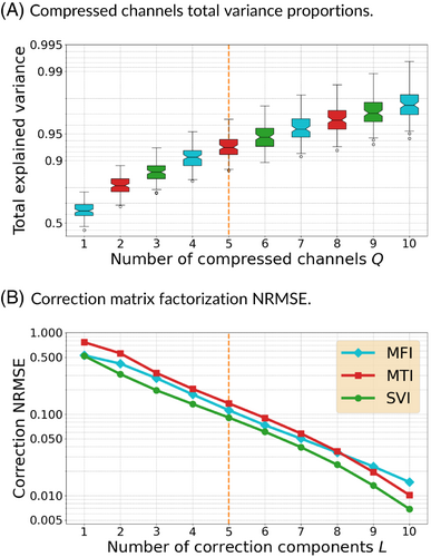
On the contrary, the SVI correction coefficients cover specific regions of the off-resonance spectrum (Figure S6). Simply using the first $L$ components, also studied hereafter, would mostly shift the data consistency focus toward low off-resonance areas that cover a much broader part of the brain images. A possibility to extend the spectrum coverage is to change the components used for data consistency over consecutive iterations. The SVI coefficients are more convenient for this, as two sets of ${L}_1$ and ${L}_2$ components with ${L}_2>{L}_1$ will share the same first ${L}_1$ components because of the orthogonality of the decomposition. This is not true for MFI and MTI methods as observed in Figures S4 and S5. It ensures that, while the first ${L}_1$ components carry the maximal amount of information, they are not redundant with the other ${L}_2-{L}_1$ components. Diverse strategies have been considered. The best performing solution updates data consistency between the first $L$ components and the following $L+1$ to $2L$ components over iterations, called ${\mathrm{SVI}}_{1/2}$ hereafter, to enforce fidelity toward either low or high off-resonance areas, respectively, in an alternated manner.

The goal is to provide improved reconstruction and correction while minimizing the processing time. $I$ , $Q$ , and $L$ linearly multiply the time with exponentially decreasing quality contributions, as shown in Figure 1 and in supplementary materials with Table S4. Our approach is therefore to reduce the reconstruction load and recover the image quality using neural networks over compressed information.

3 METHODS

3.1 Proposed pipelines

Following the recommendations from Ramzi et al.,⁴² the end-to-end NC-PDNet architecture⁴³ has been used as we consider 3D non-Cartesian SWI data. Particularly, we investigated the primal-only version where only the image domain processing is learned with an arbitrary neural network whereas data consistency is applied in k-space. However, in the context of 3D high resolution non-Cartesian and multi-coil imaging, the amount of graphics processing unit (GPU) memory required for a complete training is excessive. All or part of that memory can be moved to central processing unit CPU, but would result in a considerably longer training duration.

To address this issue, a solution often called greedy learning⁵⁶ consists in breaking down the learning process into stacks trained sequentially to avoid any restriction on the number of iterations or the network size. An ideal case would be to have stacks consisting of at least one network pass followed by a data consistency block to still learn complementary features; however, the memory requirement increases drastically at the transition between single channel image domain and multi-coil k-space data. Therefore, the simplest proposition is to exclude the data consistency from the gradient computation by training an image-to-image network as represented in Figure 2, and then only apply data consistency and repeat for each stack.

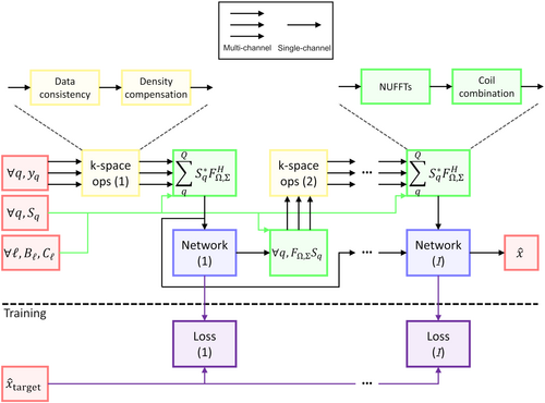
This modification requires adapting the feature originally named “memory”⁴⁰ or more recently “buffer”,⁴³ where networks could carry additional channels of information between iterations, as the additional network output channels are not all included in the backpropagation graph anymore. Instead, the network output is a single complex-valued volume but that will still be concatenated into a buffer of ${N}_B$ volumes from previous stacks to be used as input for the next stack. That way, the overall pipeline keeps the expressiveness required to learn CS-like acceleration schemes as originally suggested.⁴⁰ The main drawback compared to end-to-end training is enforcing that each stack should yield the target results rather than letting each of the independent networks build intermediate states. However, this modification allows us to train architectures with an arbitrarily high number of coils and iterations.

The different partial correction strategies based on ${F}_{\varOmega, \varSigma }$ discussed in Section 2.3 are studied within an unrolled architecture in combination with UNets in the image domain. Indeed, conventional data consistency would either enforce the off-resonance artifacts in spite of the networks, or at best would not contribute to their correction. For all of the following studies, the variables $I=5$ , $Q=5$ and $L=5$ have been retained to allow for 3D 0.6 mm isotropic corrections within 7–8 min of computing time at inference. The MFI, MTI and SVI coefficients are compared, along with the ${\mathrm{SVI}}_{1/2}$ strategy, with ${N}_B=3$ buffers and pre-computed density compensations⁵⁷ for the NUFFT operator from the gpuNUFFT¹^,⁵⁸ and pysap-mri²^,⁵⁹ packages. The residual UNets are composed of three scales, each made of convolutional blocks of three layers with kernel size of $3\times 3\times 3$ and each followed by a ReLU activation (except for the final layer). The number of filters is doubled at each 3D $2\times 2\times 2$ downscale, with 16 filters at the first scale, and vice-versa for upscales. The complex nature of the input and output volumes is handled by considering real and imaginary parts as two separate real-valued channels. All deep-learning pipelines are composed of $L=5$ independent UNets, each with 390 066 parameters with buffers and 388 338 without. They are trained for 300 epochs, resulting in 100 h long trainings for each pipeline overall, with RAdam optimizer and learning rate of $5\times {10}^{-4}$ . The minimized cost function is the sum of an L1 loss applied to complex-valued images and multiscale SSIM over the magnitude images. All training experiments were run on the Jean-Zay supercomputer over a single NVIDIA Tesla V100 GPU with 32GB of VRAM.

3.2 Dataset

A total of 123 SWI volumes were acquired on patients with non-Cartesian 3D GRE sequences at 3T (Magnetom Prisma, Siemens Healthcare, Erlangen, Germany) with a 64-channel head/neck coil array. The protocol was approved by local and national ethical committees (IRB: CRM-2111-207). Patient demographics, a study flow diagram and an illustration of SPARKLING trajectories are provided in the supplementary materials (Section S1). The dataset covers a wide range of pathologies (aneurysm, sickle cell anemia, multiple sclerosis) and off-resonance related artifact levels.

Four different variations of the recently proposed full 3D SPARKLING¹¹ sampling pattern were used, but the vast majority (n = 102) were acquired using the following parameters: A 0.6 mm isotropic resolution, a field-of-view of 24 cm in-plane (

N

= 384) over 12.5 cm (

{N}_z

= 208), a readout of

{T}_{\mathrm{obs}}=20.48

ms centered around an echo time

TE=20

ms, a repetition time

TR=37

ms. A dwell time of

\delta t=2\ \upmu \mathrm{s}

was used to balance the small number of spokes

{N}_c

= 4900, resulting in

{N}_s

= 10 240 samples per spoke. The other closely related acquisition variations are similarly described in the supplementary materials (Section S1). An acquisition time of 3 min corresponds to an acceleration factor (AF) of 17, defined as follows:

\mathrm{AF}\kern0.5em {\displaystyle \begin{array}{c}=\frac{N\times {N}_z}{N_c}.\end{array}}

(13)

The $\Delta {B}_0$ field maps were not acquired in order to avoid prolonging the exams. Instead self-estimated field maps were computed a posteriori using a recently published technique.¹⁴ To generate the ground truths, the field maps were used for model-based correction using the method described in³¹ with the SVI coefficients, resulting in approximately 8 h long reconstructions/corrections with $I=20$ , $Q=20$ and $L=20$ over a single NVIDIA Tesla V100 GPU.

The dataset was then split into training (n = 99), validation (n = 11) and testing (n = 11) sets according to balanced age, gender, weight, off-resonance pre and post-correction visibility, and pathology type and visibility distributions. Two acquisitions were excluded due to strong motion (n = 1) and insufficient off-resonance correction (n = 1) caused by braces. In both cases, the self-estimated off-resonance correction still considerably improved the images. Minor quality concerns were raised regarding skin fat artifacts (n = 6) and partially deactivated readout coils (n = 2) without causing exclusion.

Although the trainings were carried out from complex-valued to complex-valued volumes, the SWI specific processing was applied afterwards for visualization and scoring as described in.¹² The low frequencies were extracted by applying a Hanning window over the central third of k-space, before being removed from the phase image to obtain a high frequency map, subsequently normalized to produce a continuous mask. The magnitude image was multiplied five times by the mask, and a minimum-intensity projection (mIP) was computed using a thickness of 8 mm. All post-processing steps were again run on the Jean-Zay supercomputer.

3.3 Baselines

Diverse baseline models are proposed to assess the contributions of the different features involved in our pipeline. A first baseline detailed in the supplementary materials (Section S3) is given by replacing the neural networks by conventional CS reconstruction using sparsity promoting regularization in the wavelet domain (Symlet eight basis decomposed over three scales). The ${L}_1$ -norm was used for $\mathcal{R}$ function with $\lambda ={10}^{-7}$ for thresholding the wavelet coefficients. To compensate the absence of buffers to learn acceleration schemes over iterations, the FISTA⁴⁷ algorithm available in the pysap-mri package was used. The data consistency is implemented with ${F}_{\varOmega, \varSigma }$ with SVI coefficients reduced to $L=5$ . This baseline noted ${\mathrm{BASE}}_{\mathcal{R}}$ is used to determine to what extent the contribution of neural networks is critical for improved image quality.

The second baseline ${\mathrm{BASE}}_{\mathcal{C}}$ similarly replaces the correcting operator ${F}_{\varOmega, \varSigma }$ with the regular NUFFT ${F}_{\varOmega }$ while applying the same network-based regularization as the proposed pipeline.

Finally, the SVI and ${\mathrm{SVI}}_{1/2}$ pipelines were tested without buffers, along with the ${\mathrm{BASE}}_{\mathcal{C}}$ baseline. The goal was to assess that the buffer feature, modified to fit the stacked-training setup, was still relevant even without end-to-end training.

3.4 Evaluation

The results are assessed according to several criteria: Image quality, off-resonance correction and speed. The first one is commonly assessed⁶⁰ using the structural similarity index (SSIM) and the peak signal-to-noise ratio (PSNR) measures. However, parameters such as the number of coils

Q

barely contribute to off-resonance correction, as shown in Figure 3, and therefore we also provided

\Delta {B}_0

-weighted versions of SSIM and PSNR. In both cases, the voxel-wise score at position

r

was weighted by:

{w}_{\Delta {B}_0}(r)\kern0.5em {\displaystyle \begin{array}{c}=\frac{\mid \Delta {B}_0(r)\mid }{\overline{\mid \Delta {B}_0\mid }}\end{array}}

(14)

with

\overline{\mid \Delta {B}_0\mid }

the average value of the absolute

\Delta {B}_0

field map. In the case of PSNR, it corresponds to using a weighted mean-squared error (MSE) in the expression. Among those four metrics, the

\Delta {B}_0

-weighted SSIM was chosen as the primary score for this study as it relates more to the visual impact of off-resonance artifacts, followed by classic SSIM for image quality in general. Since these criteria are not defined for complex-valued data, all metrics are applied after SWI processing to also account for magnetic susceptibility information. The individual scores were then compared between pipelines for both SSIM and

\Delta {B}_0

-weighted SSIM in order to obtain

p

-values through two-sided Wilcoxon signed-rank tests, before applying a Benjamini-Hochberg correction to adjust the false discovery rate at a p-value of

p=0.05

The final aspect we focus on in this study is the computation speed of the different pipelines. The main bottleneck is the NUFFT, and has therefore been the focus for more code optimizations³^,⁴ Some other elements, such as the wavelet transform used for sparsity-promoting regularization or the computation of correcting coefficients

\left(\hat{B},\hat{C}\right)

, that are already fast in comparison but not negligible, did not benefit from similar attention. Consequently, these computations might irrelevantly change the duration. Additionally, as the proposed pipeline optimizations are solely related to the amount of individual calls to the NUFFT operator, we decided to track them as

{N}_F

to account for the numerical complexity rather than using misleading time measurements:

{N}_F\kern0.5em {\displaystyle \begin{array}{c}={N}_{F,S}+{N}_{F,R}\end{array}}

(15)

\begin{array}{rr}& \\ {}{N}_{F,S}& ={L}_S\times Q\end{array}

(16)

\begin{array}{rr}& \\ {}& \\ {}{N}_{F,R}& =L\times Q\times \left(2\times \mathcal{I}-1\right)\end{array}

(17)

with

{N}_{F,S}

the number of calls related to the sensitivity map computation, and

{N}_{F,R}

the number of calls related to image reconstruction. The sensitivity maps are systematically corrected with

{L}_S=10

components when

{F}_{\varOmega, \varSigma }

is used in Eq. (3), but not corrected at all when using

{F}_{\varOmega }

which is equivalent to

{L}_S=1

. The reconstruction consists of one iteration for initialization and

\mathcal{I}-1

iterations using data consistency. Note that the forward and adjoint calls are similarly considered for simplicity reasons, although they differ over non-Cartesian grids.

4 RESULTS

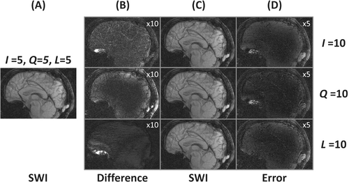
The different pipelines are compared to each other hereafter, along with an ablation study of the modified buffer feature. Additional resources are provided in the supplementary materials, and notably more exhaustive CS baselines to quantify and understand the specific contributions of varying parameters $I$ , $Q$ , and $L$ (Section S3). The number of coils $Q$ in particular, as in Figure 3, is shown to have little influence on off-resonance correction, and the coil sensitivity profiles normalized in Eq. (3) seem to have more impact on all metrics than information carried by additional coils. In contrast, increasing $L$ contributes solely to off-resonance artifacts correction while augmenting $I$ positively impacts both off-resonance and high frequency content.

4.1 Correction pipelines

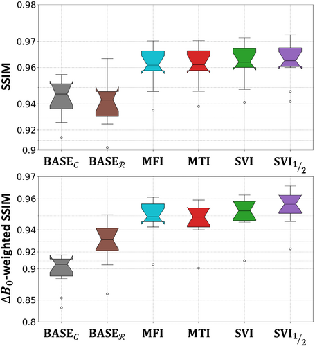
The different scores are reported in Table 1 and Figure 4, with corresponding pairwise $p$ -values in Table 2, and illustrated in Figure 5. Firstly, the baselines BASE ${\kern0em }_{\mathcal{C}}$ and BASE ${\kern0em }_{\mathcal{R}}$ in Table 1 demonstrate the expected positive contribution of a partially corrected Fourier operator ${F}_{\varOmega, \varSigma }$ against a basic model (BASE ${\kern0em }_{\mathcal{C}}$ ), and that of stacked UNets against wavelet-based regularization (BASE ${\kern0em }_{\mathcal{R}}$ ). The only statistically significant difference holds for $\Delta {B}_0$ -weighted SSIM, with a large improvement for BASE ${\kern0em }_{\mathcal{R}}$ . Therefore, the proposed UNet architecture, when combined with conventional operator ${F}_{\varOmega }$ , is not capable of correcting off-resonance effects as much as a partially correcting operator ${F}_{\varOmega, \varSigma }$ does.

TABLE 1. Scores for different correction coefficients and pipelines over the test dataset

Pipeline	Data consistency	Regularization	SSIM	PSNR	SSIM	PSNR
			Classic		$\Delta {B}_0$ -weighted
${\mathrm{BASE}}_{\mathcal{C}}$	${F}_{\varOmega }$	UNet	0.9421	33.32	0.8947	23.50
BASE ${\kern0em }_{\mathcal{R}}$	${F}_{\varOmega, \varSigma }$ (SVI)	Wavelet	0.9392	31.32	0.9249	23.33
MFI	${F}_{\varOmega, \varSigma }$ (MFI)	UNet	0.9596	34.96	0.9475	26.42
MTI	${F}_{\varOmega, \varSigma }$ (MTI)	UNet	0.9601	35.13	0.9452	26.11
SVI	${F}_{\varOmega, \varSigma }$ (SVI)	UNet	0.9613	35.24	0.9498	26.57
${\mathrm{SVI}}_{1/2}$	${F}_{\varOmega, \varSigma }$ (SVI)	UNet	0.9616	35.19	0.9541	27.31

Note: Various pipelines with $I=5$ , $Q=5$ and $L=5$ are summarized with their data consistency and regularization terms and evaluated using classic and $\Delta {B}_0$ -weighted SSIM and PSNR scores.Bold signifies best (i.e. highest) PSNR and SSIM score.

TABLE 2. Pairwise comparison p-values for all coefficients using two-sided Wilcoxon signed-rank tests on classic and

\varDelta {B}_0

-weighted SSIM scores with Benjamini-Hochberg correction

(a) Classic SSIM
	${\mathrm{BASE}}_{\mathcal{C}}$	BASE ${\kern0em }_{\mathcal{R}}$	MFI	MTI	SVI	${\mathrm{SVI}}_{1/2}$
${\mathrm{BASE}}_{\mathcal{C}}$		-	**	**	**	**
BASE ${\kern0em }_{\mathcal{R}}$	-		**	**	**	**
MFI	**	**		-	**	**
MTI	**	**	-		**	**
SVI	**	**	**	**		-
${\mathrm{SVI}}_{1/2}$	**	**	**	**	-

(a) $\varDelta {B}_0$ -weighted SSIM
	${\mathrm{BASE}}_{\mathcal{C}}$	BASE ${\kern0em }_{\mathcal{R}}$	MFI	MTI	SVI	${\mathrm{SVI}}_{1/2}$
${\mathrm{BASE}}_{\mathcal{C}}$		**	**	**	**	**
BASE ${\kern0em }_{\mathcal{R}}$	**		**	**	**	**
MFI	**	**		*	**	**
MTI	**	**	*		**	**
SVI	**	**	**	**		**
${\mathrm{SVI}}_{1/2}$	**	**	**	**	**

Note: Various pipelines with $I=5$ , $Q=5$ and $L=5$ are summarized with their data consistency and regularization terms and evaluated using classic and $\varDelta {B}_0$ -weighted SSIM and PSNR scores.
p > 0.05 .
p < 0.05 .
p > 0.005 .

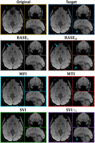
Secondly, the different correction approaches (MFI, MTI, SVI) are combined with UNets through data consistency terms. All of them show significantly higher scores than both baselines. Their $\Delta {B}_0$ -weighted SSIM score follow the same ranking as those previously observed in Figure 1B prior to image reconstruction when solving Eq. (10): the SVI coefficients reach a better score as compared to MFI (second) and MTI (third) coefficients. This suggests that none of the diverse correction approaches carried by the different coefficients are better suited than another to help UNets compensate for the missing correction.

Finally, the ${\mathrm{SVI}}_{1/2}$ pipeline improves the SVI approach with regard to $\Delta {B}_0$ -weighted SSIM, while not significantly deviating from it for classic SSIM. Exploring more components appears to guide the correction that networks alone could not achieve. This can be observed in Figure 5 near the bucco-nasal region visible with the sagittal views, where only ${\mathrm{SVI}}_{1/2}$ recovers high-frequency details consistent with the target. The additional baselines from supplementary materials (Section S3) show that the ${\mathrm{SVI}}_{1/2}$ pipeline competes with reconstruction two to three times slower depending on the evaluation criteria.

4.2 Network and model contributions

The reconstruction steps are further decomposed between data consistency and regularization in Figure 6 and illustrated in Figure 7. For both metrics, the two baselines shown in Figure 6 with brown (BASE ${\kern0em }_{\mathcal{R}}$ ) and gray (BASE ${\kern0em }_{\mathcal{C}}$ ) curves are again significantly different. The BASE ${\kern0em }_{\mathcal{R}}$ curves show a slow start with oscillations between improving data consistency and degrading regularization but with a regular progression afterwards. The oscillations are explained by the constant wavelet threshold, too large during early iterations when the overall magnitude was still too low. In contrast, the networks used in BASE ${\kern0em }_{\mathcal{C}}$ considerably improve the initialization, then followed by oscillations caused by the data consistency. Those oscillations can be explained by the off-resonance artifacts enforced through the wrong Fourier model ${F}_{\varOmega }$ but also by the sensitivity profiles altered by the normalization from Eq. (3) when reducing the number of channels $Q$ . Both are illustrated in Figure 7 with green and blue arrows respectively.

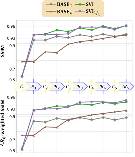
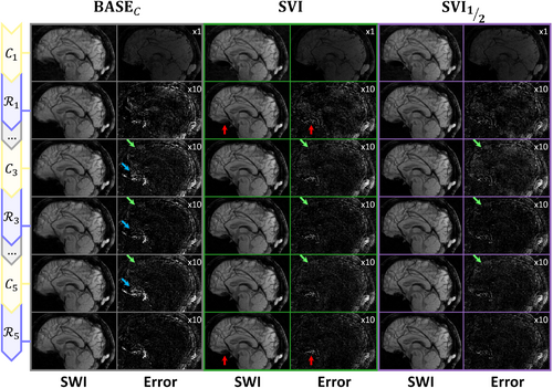
The proposed pipelines SVI and ${\mathrm{SVI}}_{1/2}$ are observed to combine a steeper initialization and better progression over iterations, but still with sensitivity-related oscillations. The ${\mathrm{SVI}}_{1/2}$ is however more robust to those as it alternates between large regions with heterogeneous sensitivities and smaller $\varDelta {B}_0$ -specific regions. Overall, the UNets appear to contribute to all three studied factors, but the striking difference between BASE ${\kern0em }_{\mathcal{C}}$ , SVI, and ${\mathrm{SVI}}_{1/2}$ pipelines suggests that networks only recover low image frequencies when correcting off-resonance. The partial correction model is therefore required in those regions, but the networks serve as an effective image pre-conditioner.

4.3 Buffer feature ablation

The main pipelines have been evaluated with and without the proposed buffer feature modified to account for stacked training, namely SVI and ${\mathrm{SVI}}_{1/2}$ along with BASE ${\kern0em }_{\mathcal{C}}$ . The different results are shown in Table 3.

TABLE 3. Ablation study of the buffer feature over different architectures on testing dataset

Pipeline	Buffers	p	SSIM	PSNR	p	SSIM	PSNR
		Classic			$\varDelta {B}_0$ -weighted
${\mathrm{BASE}}_{\mathcal{C}}$	-	-	0.9427	33.40	**	0.8979	23.69
${\mathrm{BASE}}_{\mathcal{C}}$	3	-	0.9421	33.32	**	0.8947	23.50
SVI	-	*	0.9603	35.11	*	0.9490	26.57
SVI	3	*	0.9613	35.24	*	0.9498	26.57
${\mathrm{SVI}}_{1/2}$	-	**	0.9575	34.71	**	0.9493	26.98
${\mathrm{SVI}}_{1/2}$	3	**	0.9616	35.19	**	0.9541	27.31

Note: The best performing pipelines (SVI and ${\mathrm{SVI}}_{1/2}$ ) are evaluated with and without buffers, along with the baseline ${\mathrm{BASE}}_{\mathcal{C}}$ based on the non-correcting Fourier operator ${F}_{\varOmega }$ . The classic and $\varDelta {B}_0$ -weighted scores are averaged over the testing dataset, with statistical significance assessed through pairwise two-sided Wilcoxon signed-rank tests over the SSIM scores with a global Benjamini-Hochberg correction.
p > 0.05 .
p < 0.05 .
p > 0.005 .

The baseline BASE ${\kern0em }_{\mathcal{C}}$ that combines UNets with conventional Fourier data consistency shows $\Delta {B}_0$ scores significantly worse when using the buffer feature. One interpretation could be that as consistency with corrupted brings back artifacts, as observed in Figure 7, adding memory of previous iterations only leads to a noisier learning process without additional information.

On the other hand, the ${\mathrm{SVI}}_{1/2}$ approach shows significant and large improvements with buffers, more than for the SVI pipeline. However, it should be noted that ${\mathrm{SVI}}_{1/2}$ classic scores without buffers are much lower than any other proposed pipeline, but still better than the baselines. This suggests that the exploratory correction strategy inherently degrades the overall reconstruction to advantage the off-resonance areas, but that buffer feature allows for a compensatory effect within neural networks.

5 DISCUSSION

The diverse contributions of this article are discussed hereafter. First, we compared conventional methods^29-31 to perform, to the best of our knowledge, the first partial off-resonance correction study. Second, we analyzed the deep learning contributions in a multi-parametric acceleration pipeline. Finally, we conducted a deep learning study over a fairly large in vivo dataset consisting of model-based self-estimated off-resonance corrected volumes.¹⁴

5.1 Network and model improvements

The network and model contributions when facing reduced number of iterations, compressed coils, and correction components have been studied in Section 4.

Overall, the number of coils $Q$ was observed to impact metrics by changing the sensitivity distribution superficially rather than improving the signal. Other normalization⁶¹ or coil compression methods⁶² could be explored in the future to at least balance this scoring issue. The proposed UNets appeared to mostly improve the initialization overall and help progression through the buffer feature when applying the ${\mathrm{SVI}}_{1/2}$ strategy otherwise less efficient. The latter shows how deep learning allows for more flexibility when designing hybrid algorithms. However, high-frequency details are still only recovered through model-based correction.

More elaborated strategies could be developed to distribute efficiently the correction components over iterations. Particularly, for in-out SPARKLING trajectories the MTI coefficients were shown to correlate with high/low image frequencies. A better balance between low frequencies covered by neural networks and high frequencies enforced by specifically selected correction components might produce more reliable results.

5.2 Dataset generation

The $\Delta {B}_0$ map estimation technique developed in a previous publication¹⁴ assumes the relationship between ${B}_0$ inhomogeneities and image phase to be dominant over other phase sources for large echo times (e.g., 20 ms and higher) at 3T. It allows for a simple estimate of the $\Delta {B}_0$ field map retrospectively with minimal error and no motion-related mismatch for SWI acquisitions and alike. It also avoids any assumptions on the trajectory and can, therefore, be used on any dataset matching the above-mentioned acquisition setup and providing either the raw k-space data or complex-valued MR images.

The self-estimation method has been carefully assessed during the early stages of the study, and reached our expectations. However, two other competing methods were also considered, the first by Lee et al.³⁸ through simulation from a binary mask, and the second by Patzig et al.³⁵ through non-convex optimization. The simulation method in particular has been implemented in Python but the required mask obtained from the artifacted images was suboptimal. The main advantage of those three self-estimation methods for the purpose of our proposed acceleration pipeline is to require strictly the same data. This implies that the pipeline could be efficiently applied within the clinical context and additionally improve over sessions using the same acquisitions processed through longer and dedicated procedures.

6 CONCLUSIONS

MR acquisitions based on non-Cartesian acquisitions tend to exploit longer but fewer complex readouts to reduce overall scan times but suffer more from ${B}_0$ inhomogeneities. Diverse methods exist to compensate for these artifacts, but the few non-constraining ones slow down reconstructions by an unacceptably large factor (10–20 at 3T). Deep learning techniques have been developed in the recent years, but mostly to estimate the $\Delta {B}_0$ field map which can already be self-estimated using efficient models for SWI, or to compensate for undersampling artifacts in the CS setting. The proposed approach combines partial models and deep learning to ensure data fidelity at a low computation cost when addressing off-resonance artifacts and gain in image quality. It outlines both their individual and joint contributions. The MR volumes reconstructed at inference in only 7–8 min are competing with baselines obtained in 30 min to approximate 8 h long computations, and could be further accelerated by developing new hybrid strategies. Future work might also explore the parallel aspects of the correcting models to better fit memory constraints of the GPUs, or simply include undersampling compensation through self-supervised learning methods.

ACKNOWLEDGMENTS

The concepts and information presented in this article are based on research results that are not commercially available. Future availability cannot be guaranteed. This work was granted access to the HPC resources of IDRIS under the allocation 2021-AD011011153 made by GENCI. We thank Dr. Zaccharie Ramzi and Chaithya G R for their previous works and open-source contributions. Additionally we thank Cecilia Garrec for the scientifc editing in English. Philippe Ciuciu received funding from Siemens Healthineers (France) to support this research.

ENDNOTES

Supporting Information

REFERENCES

1Pruessmann KP, Weiger M, Börnert P, Boesiger P. Advances in sensitivity encoding with arbitrary k-space trajectories. Magn Reson Med. 2001; 46: 638-651.
10.1002/mrm.1241
CAS PubMed Web of Science® Google Scholar
2Griswold MA, Jakob PM, Heidemann RM, et al. Generalized autocalibrating partially parallel acquisitions (GRAPPA). Magn Reson Med. 2002; 47: 1202-1210.
10.1002/mrm.10171
PubMed Web of Science® Google Scholar
3Lustig M, Donoho D, Pauly JM. Sparse MRI: the application of compressed sensing for rapid MR imaging. Magn Reson Med. 2007; 58: 1182-1195.
10.1002/mrm.21391
CAS PubMed Web of Science® Google Scholar
4Seiberlich N, Breuer FA, Blaimer M, Barkauskas K, Jakob PM, Griswold MA. Non-Cartesian data reconstruction using GRAPPA operator gridding (GROG). Magn Reson Med. 2007; 58: 1257-1265.
10.1002/mrm.21435
CAS PubMed Web of Science® Google Scholar
5Vasanawala SS, Alley MT, Hargreaves BA, Barth RA, Pauly JM, Lustig M. Improved pediatric MR imaging with compressed sensing. Radiology. 2010; 256: 607-616.
10.1148/radiol.10091218
PubMed Web of Science® Google Scholar
6Boyer C, Chauffert N, Ciuciu P, Kahn J, Weiss P. On the generation of sampling schemes for MRI. SIAM Imaging Sci. 2016; 9: 2039-2072.
10.1137/16M1059205
Web of Science® Google Scholar
7Luo T, Noll DC, Fessler JA, Nielsen JF. A GRAPPA algorithm for arbitrary 2D/3D non-Cartesian sampling trajectories with rapid calibration. Magn Reson Med. 2019; 82: 1101-1112.
10.1002/mrm.27801
PubMed Web of Science® Google Scholar
8Polak D, Cauley S, Huang SY, et al. Highly-accelerated volumetric brain examination using optimized wave-CAIPI encoding. J Magn Reson Imaging. 2019; 50: 961-974.
10.1002/jmri.26678
PubMed Web of Science® Google Scholar
9Lazarus C, Weiss P, Chauffert N, et al. SPARKLING: variable-density k-space filling curves for accelerated T2*-weighted MRI. Magn Reson Med. 2019; 81: 3643-3661.
10.1002/mrm.27678
PubMed Web of Science® Google Scholar
10Lazarus C, Weiss P, El Gueddari L, et al. 3D variable-density SPARKLING trajectories for high-resolution T2*-weighted magnetic resonance imaging. NMR Biomed. 2020; 33:e4349.
10.1002/nbm.4349
CAS PubMed Web of Science® Google Scholar
11Chaithya GR, Weiss P, Daval-Frérot G, Massire A, Vignaud A, Ciuciu P. Optimizing full 3D SPARKLING trajectories for high-resolution magnetic resonance imaging. IEEE Trans Med Imaging. 2022; 41: 2105-2117.
10.1109/TMI.2022.3157269
CAS PubMed Web of Science® Google Scholar
12Haacke EM, Xu Y, Cheng YCN, Reichenbach JR. Susceptibility weighted imaging (SWI). Magn Reson Med. 2004; 52: 612-618.
10.1002/mrm.20198
PubMed Web of Science® Google Scholar
13Wu Z, Mittal S, Kish K, Yu Y, Hu J, Haacke EM. Identification of calcification with MRI using susceptibility weighted imaging: a case study. J Magn Reson Imaging. 2009; 29: 177-182.
10.1002/jmri.21617
PubMed Web of Science® Google Scholar
14Daval-Frérot G, Massire A, Mailhé B, Nadar MS, Vignaud A, Ciuciu P. Iterative static ΔB₀ field map estimation for off-resonance correction in non-Cartesian susceptibility weighted imaging. Magn Reson Med. 2022; 88: 1592-1607.
10.1002/mrm.29297
PubMed Web of Science® Google Scholar
15de Graaf RA, Juchem C. B₀ Shimming Technology. Magnetic Resonance Technology; 2016: 166-207. doi:10.1039/9781782623878-00166
10.1039/9781782623878-00166
Google Scholar
16Yudilevich E, Stark H. Spiral sampling in magnetic resonance imaging-the effect of inhomogeneities. IEEE Trans Med Imaging. 1987; 6: 337-345.
10.1109/TMI.1987.4307852
CAS PubMed Web of Science® Google Scholar
17Chaithya GR, Daval-Frérot G, Massire A, et al. More-sparkling: non-Cartesian trajectories with minimized off-resonance effects. In Proceedings of the 30th Annual Meeting of ISMRM, London 2022 1611.
Google Scholar
18Gruetter R. Automatic, localized in vivo adjustment of all first-and second-order shim coils. Magn Reson Med. 1993; 29: 804-811.
10.1002/mrm.1910290613
CAS PubMed Web of Science® Google Scholar
19Aghaeifar A, Zhou J, Heule R, et al. A 32-channel multi-coil setup optimized for human brain shimming at 9.4 T. Magn Reson Med. 2020; 83: 749-764.
10.1002/mrm.27929
PubMed Web of Science® Google Scholar
20Pinho-Meneses B, Amadon A. A fieldmap-driven few channel shim coil design for MRI of the human brain. Phys Med Biol. 2021; 66:15001.
10.1088/1361-6560/abc810
PubMed Web of Science® Google Scholar
21Pinho-Meneses B, Amadon A. Physical limits to human brain B₀ shimming with spherical harmonics, engineering implications thereof. MAGMA. 2022; 35: 1-19.
PubMed Google Scholar
22Andersson JL, Skare S, Ashburner J. How to correct susceptibility distortions in spin-echo echo-planar images: application to diffusion tensor imaging. Neuroimage. 2003; 20: 870-888.
10.1016/S1053-8119(03)00336-7
PubMed Web of Science® Google Scholar
23Fritz L, Mulders J, Breman H, et al. Comparison of EPI distortion correction methods at 3T and 7T. In Proceedings of the Annual Meeting of OHBM, Hamburg 2014.
Google Scholar
24Weiger M, Pruessmann KP, Österbauer R, Börnert P, Boesiger P, Jezzard P. Sensitivity-encoded singleshot spiral imaging for reduced susceptibility artifacts in BOLD fMRI. Magn Reson Med. 2002; 48: 860-866.
10.1002/mrm.10286
CAS PubMed Web of Science® Google Scholar
25Wilm BJ, Barmet C, Gross S, et al. Single-shot spiral imaging enabled by an expanded encoding model: demonstration in diffusion MRI. Magn Reson Med. 2017; 77: 83-91.
10.1002/mrm.26493
PubMed Web of Science® Google Scholar
26Kasper L, Engel M, Barmet C, et al. Rapid anatomical brain imaging using spiral acquisition and an expanded signal model. Neuroimage. 2018; 168: 88-100.
10.1016/j.neuroimage.2017.07.062
PubMed Web of Science® Google Scholar
27Noll DC. Multishot rosette trajectories for spectrally selective MR imaging. IEEE Trans Med Imaging. 1997; 16: 372-377.
10.1109/42.611345
CAS PubMed Web of Science® Google Scholar
28Noll DC, Meyer CH, Pauly JM, Nishimura DG, Macovski A. A homogeneity correction method for magnetic resonance imaging with time-varying gradients. IEEE Trans Med Imaging. 1991; 10: 629-637.
10.1109/42.108599
CAS PubMed Web of Science® Google Scholar
29Man LC, Pauly JM, Macovski A. Multifrequency interpolation for fast off-resonance correction. Magn Reson Med. 1997; 37: 785-792.
10.1002/mrm.1910370523
CAS PubMed Web of Science® Google Scholar
30Sutton BP, Noll DC, Fessler JA. Fast, iterative image reconstruction for MRI in the presence of field inhomogeneities. IEEE Trans Med Imaging. 2003; 22: 178-188.
10.1109/TMI.2002.808360
PubMed Web of Science® Google Scholar
31Fessler JA, Lee S, Olafsson VT, Shi HR, Noll DC. Toeplitz based iterative image reconstruction for MRI with correction for magnetic field inhomogeneity. IEEE Trans Signal Process. 2005; 53: 3393-3402.
10.1109/TSP.2005.853152
Web of Science® Google Scholar
32Ostenson J, Robison RK, Zwart NR, Welch EB. Multifrequency interpolation in spiral magnetic resonance fingerprinting for correction of off-resonance blurring. Magn Reson Imaging. 2017; 41: 63-72.
10.1016/j.mri.2017.07.004
PubMed Web of Science® Google Scholar
33Man LC, Pauly JM, Macovski A. Improved automatic off resonance correction without a field map in spiral imaging. Magn Reson Med. 1997; 37: 906-913.
10.1002/mrm.1910370616
CAS PubMed Web of Science® Google Scholar
34Sutton BP, Noll DC, Fessler JA. Dynamic field map estimation using a spiral-in/spiral-out acquisition. Magn Reson Med. 2004; 51: 1194-1204.
10.1002/mrm.20079
PubMed Web of Science® Google Scholar
35Patzig F, Wilm B, Gross S, Brunner D, Pruessmann KP. Off-resonance self-correction for single-shot imaging. In Proceedings of the 28th Annual Meeting of ISMRM Virtual; 2020. p. 3400.
Google Scholar
36Patzig F, Wilm B, Pruessmann KP. Off-resonance self-correction by implicit B0-encoding. In Proceedings of the 29th Annual Meeting of ISMRM Virtual 2021 p. 666.
Google Scholar
37Salomir R, de Senneville BD, Moonen CT. A fast calculation method for magnetic field inhomogeneity due to an arbitrary distribution of bulk susceptibility. Concepts Magn Reson Part B Magn Reson Eng. 2003; 19: 26-34.
10.1002/cmr.b.10083
Web of Science® Google Scholar
38Lee SK, Hwang SH, Barg JS, Yeo SJ. Rapid, theoretically artifact-free calculation of static magnetic field induced by voxelated susceptibility distribution in an arbitrary volume of interest. Magn Reson Med. 2018; 80: 2109-2121.
10.1002/mrm.27161
PubMed Web of Science® Google Scholar
39Muckley MJ, Riemenschneider B, Radmanesh A, et al. Results of the 2020 fastmri challenge for machine learning MR image reconstruction. IEEE Trans Med Imaging. 2021; 40: 2306-2317.
10.1109/TMI.2021.3075856
PubMed Web of Science® Google Scholar
40Adler J, Öktem O. Solving ill-posed inverse problems using iterative deep neural networks. Inverse Probl. 2017; 33:124007.
10.1088/1361-6420/aa9581
Web of Science® Google Scholar
41Schlemper J, Caballero J, Hajnal JV, Price A, Rueckert D. A deep cascade of convolutional neural networks for MR image reconstruction. International Conference on Information Processing in Medical Imaging. Springer; 2017: 647-658.
10.1007/978-3-319-59050-9_51
Google Scholar
42Ramzi Z, Ciuciu P, Starck JL. Benchmarking MRI reconstruction neural networks on large public datasets. Appl Sci. 2020; 10: 1816.
10.3390/app10051816
CAS Google Scholar
43Ramzi Z, Chaithya G, Starck JL, Ciuciu P. NC-PDNet: a density-compensated unrolled network for 2D and 3D non-Cartesian MRI reconstruction. IEEE Trans Med Imaging. 2022; 41: 1625-1638.
10.1109/TMI.2022.3144619
PubMed Web of Science® Google Scholar
44Zeng DY. Acceleration of 3D Magnetic Resonance Angiography. Stanford University; 2020.
Google Scholar
45Haskell M. Deep learning field map estimation with model-based image reconstruction for off-resonance correction of brain images using a spiral acquisition. ISMRM Workshop on Data Sampling and Image Reconstruction; 2020: 43. https://web.eecs.umich.edu/∼mhask/files/Haskell_Sedona2020_poster.pdf
Google Scholar
46El Gueddari L, Lazarus C, Carrié H, Vignaud A, Ciuciu P. Self-calibrating nonlinear reconstruction algorithms for variable density sampling and parallel reception MRI. 2018 IEEE 10th Sensor Array and Multichannel Signal Processing Workshop (SAM). IEEE; 2018: 415-419.
10.1109/SAM.2018.8448776
Google Scholar
47Beck A, Teboulle M. Fast gradient-based algorithms for constrained total variation image denoising and deblurring problems. IEEE Trans Image Process. 2009; 18: 2419-2434.
10.1109/TIP.2009.2028250
PubMed Web of Science® Google Scholar
48Kim D, Fessler JA. Adaptive restart of the optimized gradient method for convex optimization. J Optim Theory Appl. 2018; 178: 240-263.
10.1007/s10957-018-1287-4
PubMed Web of Science® Google Scholar
49Maeda A, Sano K, Yokoyama T. Reconstruction by weighted correlation for MRI with time-varying gradients. IEEE Trans Med Imaging. 1988; 7: 26-31.
10.1109/42.3926
CAS PubMed Web of Science® Google Scholar
50Noll DC. Reconstruction techniques for magnetic resonance imaging. PhD thesis, Stanford University 1991.
Google Scholar
51Gerhalter T, Gast LV, Marty B, Uder M, Carlier PG, Nagel AM. Assessing the variability of 23Na MRI in skeletal muscle tissue: reproducibility and repeatability of tissue sodium concentration measurements in the lower leg at 3 T. NMR Biomed. 2020; 33:e4279.
10.1002/nbm.4279
PubMed Web of Science® Google Scholar
52Hardee JE, Phaneuf C, Cope L, Zucker R, Gearhardt A, Heitzeg M. Neural correlates of inhibitory control in youth with symptoms of food addiction. Appetite. 2020; 148:104578.
10.1016/j.appet.2019.104578
PubMed Web of Science® Google Scholar
53Buehrer M, Pruessmann KP, Boesiger P, Kozerke S. Array compression for MRI with large coil arrays. Magn Reson Med. 2007; 57: 1131-1139.
10.1002/mrm.21237
CAS PubMed Web of Science® Google Scholar
54Doneva M, Börnert P. Automatic coil selection for channel reduction in SENSE-based parallel imaging. MAGMA. 2008; 21: 187-196.
10.1007/s10334-008-0110-x
PubMed Web of Science® Google Scholar
55Zhang T, Pauly JM, Vasanawala SS, Lustig M. Coil compression for accelerated imaging with Cartesian sampling. Magn Reson Med. 2013; 69: 571-582.
10.1002/mrm.24267
CAS PubMed Web of Science® Google Scholar
56Ozturkler B, Sahiner A, Ergen T, et al. Greedy learning for large-scale neural MRI reconstruction. In NeurIPS 2021 Workshop on Deep Learning and Inverse Problems.
Google Scholar
57Pipe JG, Menon P. Sampling density compensation in MRI: rationale and an iterative numerical solution. Magn Reson Med. 1999; 41: 179-186.
10.1002/(SICI)1522-2594(199901)41:1<179::AID-MRM25>3.0.CO;2-V
CAS PubMed Web of Science® Google Scholar
58Knoll F, Schwarzl A, Diwoky C, Sodickson DK. gpuNUFFT-an open source GPU library for 3D regridding with direct Matlab interface. In Proceedings of the 22nd Annual Meeting of ISMRM Milan, Italy 2014 4297.
Google Scholar
59El Gueddari L, Chaithya G, Ramzi Z, et al. PySAP-MRI: a python package for MR image reconstruction. In ISMRM Workshop on Data Sampling and Image Reconstruction, Sedona 2020.
Google Scholar
60Hore A, Ziou D. Image quality metrics: PSNR vs. SSIM. In 2010 20th International Conference on Pattern Recognition IEEE; 2010, pp. 2366–2369.
Google Scholar
61Herterich R, Sumarokova A. Coil Sensitivity Estimation and Intensity Normalisation for Magnetic Resonance Imaging (Dissertation). KTH Royal Institute of Technology; 2019 Retrieved from http://urn.kb.se/resolve?urn=urn:nbn:se:kth:diva-263149
Google Scholar
62Cole E, Meng Q, Pauly J, Vasanawala S. Learned compression of high dimensional image datasets. In Proceedings of the IEEE/CVF Conference on Computer Vision and Pattern Recognition; 2022, pp. 1748–1752.
Google Scholar

Citing Literature

Volume90, Issue4

October 2023

Pages 1431-1445

This article also appears in:

Machine Learning and AI

Deep learning-assisted model-based off-resonance correction for non-Cartesian SWI

Abstract

Purpose

Theory

Methods

Results

Conclusion

1 INTRODUCTION

2 THEORY

2.1 Image reconstruction

2.2 Signal correction

2.3 Accelerated reconstruction and correction

3 METHODS

3.1 Proposed pipelines

3.2 Dataset

3.3 Baselines

3.4 Evaluation

4 RESULTS

4.1 Correction pipelines

4.2 Network and model contributions

4.3 Buffer feature ablation

5 DISCUSSION

5.1 Network and model improvements

5.2 Dataset generation

6 CONCLUSIONS

ACKNOWLEDGMENTS

ENDNOTES

Supporting Information

REFERENCES

Citing Literature

Figures

References

Information

About Wiley Online Library

Help & Support

Opportunities

Connect with Wiley

Deep learning-assisted model-based off-resonance correction for non-Cartesian SWI

Abstract

Purpose

Theory

Methods

Results

Conclusion

1 INTRODUCTION

2 THEORY

2.1 Image reconstruction

2.2 Signal correction

2.3 Accelerated reconstruction and correction

3 METHODS

3.1 Proposed pipelines

3.2 Dataset

3.3 Baselines

3.4 Evaluation

4 RESULTS

4.1 Correction pipelines

4.2 Network and model contributions

4.3 Buffer feature ablation

5 DISCUSSION

5.1 Network and model improvements

5.2 Dataset generation

6 CONCLUSIONS

ACKNOWLEDGMENTS

ENDNOTES

Supporting Information

REFERENCES

Citing Literature

Figures

References

Related

Information