Volume 89, Issue 5 pp. 1707-1727

RESEARCH ARTICLE

Open Access

Quantification of MR spectra by deep learning in an idealized setting: Investigation of forms of input, network architectures, optimization by ensembles of networks, and training bias

Rudy Rizzo,

Rudy Rizzo

orcid.org/0000-0003-4572-5120

MR Methodology, Department for Diagnostic and Interventional Neuroradiology, University of Bern, Bern, Switzerland

Department for Biomedical Research, University of Bern, Bern, Switzerland

Translational Imaging Center (TIC), Swiss Institute for Translational and Entrepreneurial Medicine, Bern, Switzerland

Graduate School for Cellular and Biomedical Sciences, University of Bern, Bern, Switzerland

Search for more papers by this author

Martyna Dziadosz,

Martyna Dziadosz

MR Methodology, Department for Diagnostic and Interventional Neuroradiology, University of Bern, Bern, Switzerland

Department for Biomedical Research, University of Bern, Bern, Switzerland

Translational Imaging Center (TIC), Swiss Institute for Translational and Entrepreneurial Medicine, Bern, Switzerland

Graduate School for Cellular and Biomedical Sciences, University of Bern, Bern, Switzerland

Search for more papers by this author

Sreenath P. Kyathanahally,

Sreenath P. Kyathanahally

orcid.org/0000-0002-7399-8487

Department of System Analysis, Integrated Assessment and Modelling, Data Science for Environmental Research Group, EAWAG, Dübendorf, Switzerland

Search for more papers by this author

Amirmohammad Shamaei,

Amirmohammad Shamaei

orcid.org/0000-0001-8342-3284

Institute of Scientific Instruments of the Czech Academy of Sciences, Brno, Czech Republic, Brno, Czech Republic

Department of Biomedical Engineering, Brno University of Technology, Brno, Czech Republic

Search for more papers by this author

Roland Kreis,

Corresponding Author

Roland Kreis

[email protected]

orcid.org/0000-0002-8618-6875

MR Methodology, Department for Diagnostic and Interventional Neuroradiology, University of Bern, Bern, Switzerland

Department for Biomedical Research, University of Bern, Bern, Switzerland

Graduate School for Cellular and Biomedical Sciences, University of Bern, Bern, Switzerland

Correspondence

Roland Kreis, MR Methodology, Department for Diagnostic and Interventional Neuroradiology, University of Bern, Bern, Switzerland.

Email: [email protected]

Search for more papers by this author

Rudy Rizzo,

Rudy Rizzo

orcid.org/0000-0003-4572-5120

MR Methodology, Department for Diagnostic and Interventional Neuroradiology, University of Bern, Bern, Switzerland

Department for Biomedical Research, University of Bern, Bern, Switzerland

Translational Imaging Center (TIC), Swiss Institute for Translational and Entrepreneurial Medicine, Bern, Switzerland

Graduate School for Cellular and Biomedical Sciences, University of Bern, Bern, Switzerland

Search for more papers by this author

Martyna Dziadosz,

Martyna Dziadosz

MR Methodology, Department for Diagnostic and Interventional Neuroradiology, University of Bern, Bern, Switzerland

Department for Biomedical Research, University of Bern, Bern, Switzerland

Translational Imaging Center (TIC), Swiss Institute for Translational and Entrepreneurial Medicine, Bern, Switzerland

Graduate School for Cellular and Biomedical Sciences, University of Bern, Bern, Switzerland

Search for more papers by this author

Sreenath P. Kyathanahally,

Sreenath P. Kyathanahally

orcid.org/0000-0002-7399-8487

Department of System Analysis, Integrated Assessment and Modelling, Data Science for Environmental Research Group, EAWAG, Dübendorf, Switzerland

Search for more papers by this author

Amirmohammad Shamaei,

Amirmohammad Shamaei

orcid.org/0000-0001-8342-3284

Institute of Scientific Instruments of the Czech Academy of Sciences, Brno, Czech Republic, Brno, Czech Republic

Department of Biomedical Engineering, Brno University of Technology, Brno, Czech Republic

Search for more papers by this author

Roland Kreis,

Corresponding Author

Roland Kreis

[email protected]

orcid.org/0000-0002-8618-6875

MR Methodology, Department for Diagnostic and Interventional Neuroradiology, University of Bern, Bern, Switzerland

Department for Biomedical Research, University of Bern, Bern, Switzerland

Graduate School for Cellular and Biomedical Sciences, University of Bern, Bern, Switzerland

Correspondence

Roland Kreis, MR Methodology, Department for Diagnostic and Interventional Neuroradiology, University of Bern, Bern, Switzerland.

Email: [email protected]

Search for more papers by this author

First published: 19 December 2022

https://doi.org/10.1002/mrm.29561

Citations: 5

Click here for author-reader discussions

Funding information: H2020 Marie Skłodowska-Curie Actions, Grant/Award Number: 813120; Nvidia, Swiss National Science Foundation, Grant/Award Number: 320030-175984

Share a link

Email
Wechat
Bluesky

Abstract

Purpose

The aims of this work are (1) to explore deep learning (DL) architectures, spectroscopic input types, and learning designs toward optimal quantification in MR spectroscopy of simulated pathological spectra; and (2) to demonstrate accuracy and precision of DL predictions in view of inherent bias toward the training distribution.

Methods

Simulated 1D spectra and 2D spectrograms that mimic an extensive range of pathological in vivo conditions are used to train and test 24 different DL architectures. Active learning through altered training and testing data distributions is probed to optimize quantification performance. Ensembles of networks are explored to improve DL robustness and reduce the variance of estimates. A set of scores compares performances of DL predictions and traditional model fitting (MF).

Results

Ensembles of heterogeneous networks that combine 1D frequency-domain and 2D time-frequency domain spectrograms as input perform best. Dataset augmentation with active learning can improve performance, but gains are limited. MF is more accurate, although DL appears to be more precise at low SNR. However, this overall improved precision originates from a strong bias for cases with high uncertainty toward the dataset the network has been trained with, tending toward its average value.

Conclusion

MF mostly performs better compared to the faster DL approach. Potential intrinsic biases on training sets are dangerous in a clinical context that requires the algorithm to be unbiased to outliers (i.e., pathological data). Active learning and ensemble of networks are good strategies to improve prediction performances. However, data quality (sufficient SNR) has proven as a bottleneck for adequate unbiased performance—like in the case of MF.

1 INTRODUCTION

MR Spectroscopy (MRS) provides a noninvasive means for extracting biochemical profiles from in vivo tissues. Metabolites are encoded with different resonance frequency patterns, and their concentrations are directly proportional to the signal amplitude.^{1, 2} Metabolite quantification is traditionally based on model fitting (MF), where a parameterized model function is optimized to explain the data via a minimization algorithm. Metabolite parameters are usually estimated by a nonlinear least-squares fit (either in time or frequency domain) using a known basis set of the metabolite signals.³ However, despite various proposed fitting methods,^3-7 robust, reliable, and accurate quantification of metabolite concentrations remains challenging.⁸ The major problems influencing the quantitative outcome are: (1) overlapping spectral patterns of metabolites, (2) low SNR, and (3) unknown background signals and line shape (no exact prior knowledge). Therefore, the problem is ill-posed, and current methods address it with different regularizations and constraint strategies (e.g., parameter bounds, penalizations, choice of the algorithm), with discrepancies in the results from one method to another.⁹

Supervised deep learning (DL) utilizes neural networks to discover essential features embedded in large data sets and to determine complex nonlinear mappings between inputs and outputs.¹⁰ Thus, DL does not require any prior knowledge or traditional assumptions. Given the success of the method in different areas,^10-14 DL has been introduced into MRS as an alternative to conventional methods.^15-22 Quantification of MRS datasets has been explored as follows: (1) DL algorithms identify datasets' features and either help reduce the parameter space dimension or set reliable starting conditions for the fit (i.e., combining knowledge on the physics with DL). It showed rapid spectral fitting of a whole-brain MRSI datasets.²³ (2) Convolutional neural networks (CNNs) have been deployed to investigate combinations of spectral input of edited human brain MRS, which showed improved accuracy of straight metabolite quantitation when compared to traditional MF techniques.²⁴ (3) Regression CNNs have been used to mine the real part of rat brain spectra to predict highly resolved metabolite basis set spectra with intensities proportional to the concentrations of the contributions,¹⁷ with results comparable to traditional MF approaches and showing readiness for (pre)clinical applications.²² (4) Targeting localized correlated spectroscopy (L-COSY) datasets, DL algorithms have reported faster data reconstruction and quantification compared to alternative acceleration techniques.¹⁶

Nevertheless, despite the reported equivalence in quantitation performance compared to traditional MF,^{14, 17, 22, 23} questions arise concerning the robustness of DL algorithms. A robust use within a clinical MRS context requires the algorithm to be unbiased also for pathological spectra. In imaging, DL has shown excellent performance for classification or segmentation tasks but may suffer from inherent weaknesses in subsets of representative outlier samples.^{11, 25} DL architectures for MRS quantitation have mostly been investigated for sample distributions of near-healthy spectral metabolite content. Hence, it can be suspected that high accuracy and precision are mainly found when DL is deployed for new entries of similar near-normal types. However, inaccurate estimates may result for tests with atypical datasets.²⁶ Here, strongly variable metabolite concentrations that vary uniformly and independently over the entire plausible parameter space are used in the training set. This mimics the full range from healthy to strongly pathological spectra, that is, the full complexity of a clinical setup.

MRS signals are acquired in time domain but viewed in frequency domain. Traditional MF works in either of the two equivalent domains, and fit packages may allow the user to switch from one to the other for fitting and viewing. However, DL architectures for MRS quantification have mainly explored the frequency domain, mostly motivated by the reduced overlap between the constituting metabolite signals. Spectrograms¹⁸ present an extension into a simultaneous time/frequency domain representation and offer a 2D signal support that matches the input format for the original usage of CNN algorithms in computer vision. This work introduces a dedicated high-resolution spectrogram calculation focusing on signal-rich areas in both domains to be used as input for different CNN architectures. They are compared to other inputs and networks, inspired by previous MRS publications. Specifically, 24 network designs are investigated with differing input–output dataset types with a combined focus on depth (i.e., number of layers) and width (i.e., number of nodes/kernels) of the networks. This focus was motivated by the fact that the exploitation of spectrograms in deep learning has shown top-notch performance for speech and audio processing when deploying architectures with few layers and large convolutional kernels.^27-29 Moreover, wide and shallow networks are more suitable to detect simple and small but fine-grained features. In addition, they are easier and faster to train.³⁰ Network linearity (i.e., activation function) and locality (i.e., kernel size) are also investigated.

Besides investigating multiple architectures and input formats, two established main strategies for improving the outcome of predictions are also explored: active learning³¹ (data augmentation for critical types of spectra) and ensemble learning^{32, 33} (combination of outputs from multiple architectures).

Active learning can improve labeling efficiency,^{31, 34, 35} where the learning algorithm can interactively select a subset of examples that needs to be labeled. This is an iterative process where (1) the algorithm selects a subset of examples; (2) the subset is provided with labels; and (3) the learning method is updated with the new data.³⁶ Uncertainty sampling³⁷ is a specific strategy used in active learning that prioritizes selecting examples whose predictions are more uncertain (i.e., targeted data augmentation). Because these cases are usually close to the class separation boundaries, they contain most of the information needed to separate different classes.^{38, 39} In different applications, uncertainty sampling has been shown to improve the effectiveness of the labeling procedure significantly.^{34, 35, 37, 40}

DL algorithms are sensitive to the specifics of the training.⁴¹ Hence, they usually find a different set of weights each time they are trained, producing different predictions.¹⁰ A successful approach for reducing the variance is to train multiple networks instead of one and combine their predictions.⁴¹ This is called ensemble learning, where the model generalization is maintained, but predictions improve compared to any of the single models.³³ From a range of different techniques,^42-44 here, stacking of models is implemented.³²

To evaluate pros and cons of all these approaches, in silico ground truth (GT) knowledge is used (and hence no in vivo data was included in this evaluation) to assess performances via a dedicated set of metrics based on bias and SD. The CNN-predicted distributions of concentration are then compared to those from traditional MF. Furthermore, to emphasize the analysis at the core of the quantification task, the focus is placed on an idealized simulated setting with typical single-voxel spectra that have been preprocessed to eliminate phase as well as frequency drifts.³ This assumption aims at (1) freeing the MF algorithm from problems with local χ² minima and (2) designing DL models optimized for the quantification task only.

2 METHODS

2.1 Simulations

This work is based on in silico simulations. A dataset of 22,500 entries was randomly split into 18,000 for training, 2000 for validation, and 2500 for testing. Larger dataset sizes are also explored, see section 2.4.

2.1.1 MR spectra

Brain spectra were simulated using actual RF pulse shapes for 16 metabolites at 3 T using Vespa⁴⁵ for a semi-LASER⁴⁶ protocol with TE = 35 ms, a sampling frequency of 4 kHz, and 4096 datapoints.

Further specifics of the simulations include: (1) Voigt line shapes, (2) metabolite concentration range, (3) addition of macromolecular background signal (MMBG), (4) noise generation, and (5) spectrum or spectrogram calculation.⁴⁷ Metabolite concentrations vary independently and uniformly between 0 and twice a normal reference concentration for healthy human brain.^{1, 48-50} Maximal concentrations in mM units—NAA 25.8, tCr (1:1 sum of creatine + phosphocreatine spectra): 18.5, mI (myo-inositol): 14.7, Glu (glutamate): 20, Glc (glucose): 2, NAAG (N-acetylaspartylglutamate): 2.8, Gln (glutamine): 5.8, GSH (glutathione): 2, sI (syllo-inositol): 0.6, Gly (glycine): 2, Asp (aspartate): 3.5, PE (phosphoethanolamine): 3.3, Tau (taurine): 2, Lac (lactate): 1, and GABA (γ-aminobutyric acid): 1.8. The concentration for tCho (1:1 sum of glycerophosphorylcholine + phosphorylcholine spectra) ranges from 0 to 5 mM to mimic tumor conditions.⁵¹ A constant downscaled water reference (64.5 mM) is added at 0.5 ppm to ease quantitation. Metabolite T₂s in ms (and hence Lorentzian broadening) are fixed to reference values from literature—tCr (CH₂): 111, tCr (CH₃): 169, NAA (CH₃): 289, and all other protons: 185.^{49, 52-54} MMBG content, shim, and SNR mimicked in vivo acquisitions and varied independently and uniformly (time-domain water referenced SNR 5–40, Gaussian shim 2–5 Hz, MMBG amplitude ±33%). The MMBG pattern was simulated as a sum of overlapping Voigt lines as reported in Refs. 49 and 55 (Figure 1A).

Details are in the caption following the image — **FIGURE 1**
Open in figure viewer PowerPoint

Illustration of input formats. (A) Samples of spectra, real part, view of the central 1024 points. (B) Spectrogram computation via short-time Fourier transform. Specifically, in datapoints units (corresponding to time and frequency resolution of 0.25 ms and 1 Hz, respectively): S = 4096, Z = 6000, W = 1024, Ov = 1000, ZW = 1024. Zero-filling is tuned to select the relevant part of the spectrum with W = 1024 datapoints. (C) (Left) Arrangement on a 2D frame of short-time Fourier transforms over time bins. Color code reference to windows in part (B). A truncation at 32 bins (200 ms) in time domain is used to limit the matrix space, given an almost complete ${\mathrm{T}}_2^{\ast }$ relaxation of the FID at that point. (C) (Middle) Diagonal undersampling reduces the vertical (frequency domain) matrix size. Size reduction is about a factor N = 8. (C) (Right) Undersampled spectrogram: 128 × 32 datapoints. (D) Example of constructed spectrogram matrix. FFT, fast Fourier transform; S, support of the signal; Ov, window overlap; W, Hamming window size; Z, zero filling; ZW, truncated support of zero-filled FFT.

2.1.2 Spectrograms

A spectrogram is a complex 2D representation of a spectrum, where frequencies vary with time: Every image column represents the frequency content of a particular time portion of the FID. Time information is binned along every row of the image. It is calculated via application of a short-time Fourier transform,¹⁸ where, depending on the size of the Fourier analysis window, different levels of frequency and time resolution can be achieved. A long window size modulated via zero-filling combined with a small overlap interval is chosen to increase frequency resolution and minimize the expense of time resolution (Figure 1B). Diagonal downsampling is designed to reduce the spectrogram size, keeping the original resolution grid at least as part of the time-frequency information on consecutive bins and reducing the spectrogram size (Figure 1C) to allow reasonable computation time for a CNN architecture (i.e., 128 frequency bins × 32 time bins) (Figure 1D).

2.2 Design and training of CNN architectures

A total of 24 different CNN architectures combined with different spectroscopic input representations are compared for MRS metabolite quantification. Current state-of-the art networks have been taken as reference models and adapted to the purpose and datasets used.

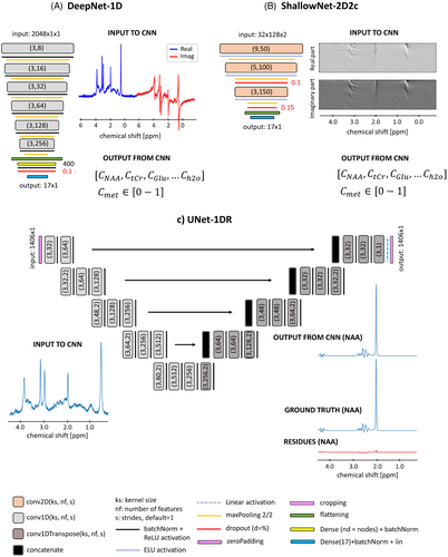
Scripts were written in Python⁵⁶ using Keras library⁵⁷ on a Tensorflow⁵⁸ backend. Code ran on either of three graphic-processing units (GPUs; NVIDIA [Santa Clara, USA] Titan Xp, Titan RTX, or GeForce RTX 2080 Ti) or Google [Mountain View, USA] Colaboratory.⁵⁹ Samples of the design are reported in Figure 2. Overall network designs are given in Table S1; Figures S1, S2, S3, S4, S5; and Text S1.

2.2.1 Architectures for straight numeric quantification of concentrations

A total of 22 architectures were fed with 1D (spectra) or 2D (spectrograms) input and mapped as output a vector of 17 normalized concentrations (i.e., in [0–1] interval) of 16 metabolites and the water reference, as listed in Table S1. Networks fed with 1D input exploit one channel with truncated spectra of 1024 datapoints from −0.5 to +6 ppm with concatenated real and imaginary parts (i.e., 2048 × 1 × 1 datapoints, Figure 2A). Networks fed with 2D input can either be configured in two channels (real and imaginary components of the spectrogram, 32 × 128 × 2 datapoints) or one channel (real and imaginary components concatenated, 64 × 128 × 1 datapoints, Figure 2B).

Five networks receive 1D input: two deep convolutional neural networks (DeepNet),⁶⁰ two residual networks (ResNet)⁶¹ and one inception network (InceptionNet).^62-64

This work investigates deep and shallow architectures either exploiting large or small convolutional kernel sizes. A total of 10 networks receive two-channel spectrograms as input. Given the limited size of the input FOV, the architecture is limited to be shallow (i.e., pooling operations to downsampling features directly following a convolutional layer are limited). However, a deeper architecture with multiple convolutional operations with sparse pooling is also compared. A further comparison is performed regarding the optimal activation function, comparing batch normalization + rectified linear unit (ReLU) versus exponential linear unit (ELU).^{65, 66} Seven networks receive one-channel spectrograms as input. With this configuration, deeper architectures are explored: two DeepNets, four ResNets, and one InceptionNet.

Architectures are analyzed either in a preconfigured parameter state or in a parameter space that had been optimized via Bayesian hyperparameterization.⁶⁷ The optimization procedure is given in Text S1. In addition, to limit biases around zero for small concentrations,⁶⁸ all network designs are characterized by a final layer with linear activation, allowing the prediction of negative concentrations.

2.2.2 Architectures for estimation of metabolite base spectra

1D input (real part only, 0–4.7 ppm, 1406 × 1 × 1 datapoints after zero-filling of original FID) was used to input and output to/from the CNNs. U-Net architectures⁶⁹ analogous to those of Ref. 22 are implemented here to map the ideal high-resolved noiseless base spectrum of a target metabolite as output. CNNs are trained one by one for each metabolite such that each CNN filters out signals only from the designated target metabolite. A base U-Net design (Figure 2C) is optimized for individual metabolites as follows:

1. UNet-1DR-hp : A total of 17 different networks with the same base architecture but adapted weights for each metabolite;
2. Unet-1DR-hp-met: A total of 17 different networks with adapted Bayesian-optimized architecture and weights for each metabolite.

Configurations are reported in Figure S5. First, metabolite concentrations are evaluated by feeding an input spectrum to the 17 metabolite-specific CNNs. Integration of the predicted metabolite base spectrum is then referenced to the integrated water reference to produce concentrations for a fully automated quantification pipeline.²²

2.2.3 Training

Training and validation sets were randomly assigned for training the CNN on a maximum of 200 epochs with batch normalization of 50. The adaptive moment estimation algorithm (ADAM)⁷⁰ was used with dedicated starting learning rates for each network.^{71, 72} The loss function was the mean-squared error (MSE). Visualization of training and validation loss over epochs combined with implementing an early-stopping criterion monitoring minimization of validation loss with patience = 10 has been used for tuning the network parameter space.⁵⁷ Training time and test loss function are listed in Table S1.

2.2.4 Evaluation

Regression plots mapping GT concentrations versus CNN predicted concentrations from the whole test set are taken as indicators of the network's prediction performance. Four scores are defined:

• a (slope of the regression line): must be close to 1 for ideal mapping of concentrations over the whole range of simulated metabolite content;
• q (intercept of the regression line, mM): must be close to 0 to minimize prediction offsets/biases;
• ${R}^2$ (coefficient of determination): must be close to 1 to assess full model explanation of the variability of the data;
• $\sigma$ (RMS error [RMSE] of prediction vs. GT, mM): as low as possible. However, expected to be comparable to Cramer Rao Lower Bounds (CRLBs) from MF.⁷³

To easily compare different networks and input setups quantitatively in the Results section, these scores or combinations thereof have been used. The combinations are referred to as concise scores: $a\cdot {R}^2$ as measure of linearity, $\sigma$ to compare with CRLBs. q was excluded because it is mostly negligible.

2.3 Influence of inclusion of water reference peak

For the evaluation of the potential benefit of including a water reference peak, two slightly different ShallowNet-2D2c-hp networks are compared. Network A outputs 17 neurons (16 metabolites and water), whereas network B outputs 16 neurons only (no water output). Two adapted datasets are used for the investigation, one with (dataset A), and one without (dataset B) downscaled water reference at 0.5 ppm. Metabolite concentrations are calculated for both cases (assuming known water content in case A). Networks have been independently trained five times to monitor network variability over multiple trainings.

2.4 Active learning and dataset size

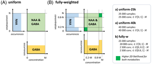
In this part, data augmentation techniques to smartly generate training sets are investigated. Subsets with 5000 new entries of the dataset where predictions scored worst are defined: specific subsets of spectrally weakly represented metabolites in either very low or very high concentrations and spectra with low SNR. New weighted datasets of 25,000 entries (20,000 training – 5000 validation set) or 40,000 entries (35,000 training – 5000 validation set) are generated (example in Figure 3, full description in Figure S6). Datasets with matching size and the testing set are kept unchanged from the previous simulation, thus with uniformly distributed concentrations and SNR. ShallowNet-2D2c-hp is selected as architecture and trained 10 times with a given augmented training set to minimize training variance.

Complementarily, given the network trained on a uniform span of concentrations, active learning is investigated in the testing phase on three different test sets where concentrations are clipped to a progressively smaller range of 20%–80%, 20%–80% with SNR >20, and 40%–60% concentration range relative to the training set.

2.5 Ensemble of networks

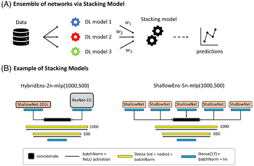
In this section, ensembles of networks are implemented via stacking of models.³² This consists of designing a DL architecture called stacking model (a multilayer perceptron (MLP) with two hidden layers is selected for this case) that will take as input the combination of a given number of independently pretrained models. The stacking model aims at weighting predictions from single models. It is trained using the same training and validation sets used to train single models while keeping the weights of the pretrained input models fixed. Three different ensembles are investigated: ShallowEns-5n groups five identical ShallowNet-2D2c-hp architectures, whereas HybridEns tests heterogeneous inputs grouping either two or 10 different networks (ShallowNet-2D2c-hp and ResNet-1D-hp) (Figure 4).

2.6 Model fitting

Spectra are fitted using FiTAID⁷ given its top performance in the ISMRM fitting challenge⁹ and to be expected for the spectra as used in the current setup (in particular, without undefined spurious baseline). The model consists of a linear combination of the metabolite base spectra with Voigt lineshape, where the Lorentzian component was kept fixed at the known GT value. The areas of the metabolites are restricted in a range corresponding to [ $-0.5+2.5\ \mu$ ], where μ is the average concentration in the testing set distribution (i.e., the normal tissue content). These bounds mimic the effective boundaries of the DL algorithms. CRLBs are used as a precision measure⁷⁴ and are considered for three subgroups of the testing set (high [SNR > 28.4], medium [16.7 < SNR < 28.4], and low [SNR < 16.7] relative SNR, respectively).

3 RESULTS

3.1 S1Metabolite quantification referenced to the downscaled water peak

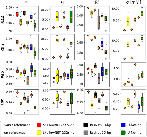
As illustrated for three different networks, Figure 5 shows that CNN predictions perform better if the spectra are referenced to a downscaled water peak: Regression slope a and ${R}^2$ are closer to 1; $\sigma$ is appreciably lower. Moreover, the spread of the scores is on average reduced, displaying improved stability over multiple trainings. Extended results are presented in Figures S7 and S8.

3.2 Network design

Figure 6 reports CNN predictions versus GT values of a ResNet-1D-hp architecture for nine metabolites (see Figures S9 and S10 for extended results on 16 metabolites or different CNN architecture). Distributions of GT and predicted values are displayed for the test set (as for all results). Predictions relate very well to the GT for well-represented metabolites (top row). However, for metabolites with lower relative SNR, predicted distributions of concentrations tend to be less uniform and are biased toward average values of the GT distributions. Thus, concentrations at distribution boundaries are systematically mispredicted, particularly for low SNR. This is reflected in lower $a$ and ${R}^2$ values and higher σ. Figures S11 and S12 include a comparison of multiple networks via bar graphs (which are ill-suited to express the systematic bias) and a plot of distributions of predictions.

The performance of all networks and fitting models for nine metabolites is reported in Figure 7 via a 2D plot of the concise scores

a\cdot {R}^2

and

\sigma

(see Figure S13 for extended results on 16 metabolites). Top performance corresponds to the top-left corner where

a\cdot {R}^2

approaches 1 and

\sigma

is low. Metabolites can roughly be divided into three groups:

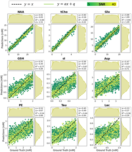
1. Well-represented metabolites: NAA, tCho, tCr, mI, Glu with averaged DL scores $a\cdot {R}^2>0.80$ and $\sigma$ < 15%, as well as MF scores $a\cdot {R}^2>0.95$ and $\sigma <10\%$ ;
2. Medium-represented metabolites: Glc, NAAG, Gln, GSH with averaged DL scores $0.50<a\cdot {R}^2<0.75$ and $20\%<\sigma <35\%$ , as well as MF scores $0.75<a\cdot {R}^2<0.90$ and $15\%<\sigma <35\%$ ;
3. Weakly represented metabolites: sI, Gly, Asp, PE, Tau, Lac, GABA with averaged DL scores $a\cdot {R}^2<0.40$ and average $\sigma >35\%$ , as well as MF scores $a\cdot {R}^2<0.65$ and $\sigma >35\%$ .

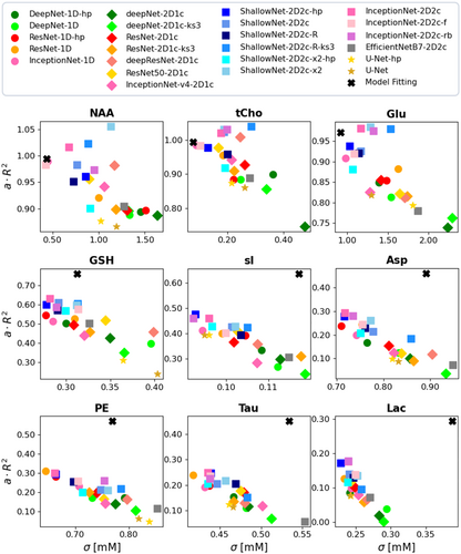
Overall, multiple DL networks perform similarly, but some general differences are noteworthy. Optimized spectrogram representation via two channels combined with a shallow architecture (i.e., dark blue squares) is found to be well suited for MRS quantification, showing mostly better performances than alternative deeper designs (i.e., light blue, pink, and gray squares), with one-channel designs (diamonds) or 1D spectra as signal representation (circles). Benefits are evident for medium and weakly represented metabolites. Performances of direct quantification and two-step quantification via base spectrum prediction followed by integration (stars) are similar. MF is found superior to DL for all medium- and weakly represented metabolites with significant average improvements for $a\cdot {R}^2.$ However, σ tends to be higher for many cases. A more detailed presentation of performance is given in Figures S14 and Text S2.

Figure 8 displays plots of prediction errors (i.e., Δ = prediction−GT) and their spread σ as a functionof SNR and shim for tCho, NAAG, and sI. Prediction uncertainties increase with noise level approximately linearly with 1/SNR and reach a plateau for weakly represented metabolites when the spread represents essentially the whole training range. No dependence on shim is apparent for the investigated range.

3.3 Dataset size, active learning, and ensembles of networks

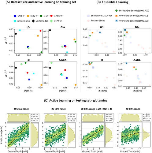
Figure 9 reports on performance improvements by active learning in training phase and dataset sizing (part 9A) as well as by using an ensemble of networks (part 9B) for four metabolites as reflected by concise scores. Outcomes of emulated active learning approaches in limiting the testing sets are illustrated through regression plots for Gln in Figure 9C. Detailed comparisons for 16 metabolites are given in Figure S15, Table S2, Table S3, Figure S16, and Table S4.

3.3.1 Dataset size

The performance showed moderate improvements for most metabolites when dataset size was increased from 25,000 to 40,000 samples (Figure S9).

3.3.2 Active learning

Dataset augmentation to favor training with combinations of low or high concentrations of weakly represented metabolites (see Figure S6B–S6D) does not substantially improve performance (Figure 9A, Figure S15, Table S2). Mild improvements (<6% for a, q, ${R}^2$ and $\sigma$ ) are seen for GABA and sI, respectively, when exploiting metabolite-specifically augmented datasets (GABA-w, sI-w). Increased dataset size combined with data augmentation to favor high and low concentrations of different metabolites (GSPT-w) moderately improves performances for the augmented metabolites (GABA, sI, PE, Tau). It also extends mild improvements to medium- to weakly represented metabolites that have not undergone data augmentation (e.g., Lac, Gly, Gln). A dataset that is strongly weighted toward extreme combinations of low or high concentration for all metabolites (fully-w) or a dataset weighted toward low SNR (SNR-w) deteriorated performances.

Clipping the test set to 20%–80% or 40%–60% of the concentration range in training renders improved performances (on average a + 4.5%, q−10.2%, $\sigma$ −23.9% and a + 4%, q−37.5%, $\sigma$ −36.2%, respectively), which is even enhanced further when the testing set includes samples with higher SNR (on average a + 15.4%, q−45.4%, $\sigma$ −36.2%). Given the limited range on the y-axis, ${R}^2$ is less representative (Figure 9C, Table S3).

3.3.3 Ensemble of networks

Ensembles of Bayesian-optimized networks show consistent and relevant $a\cdot {R}^2$ improvements for medium- to weakly represented metabolites without deteriorating performance for well-defined metabolites. A hybrid ensemble outperforms the ensemble of networks of the same type. The performance of the ensemble increases with the number of combined networks (Figures 9B, S16) (Table S4).

3.4 CNN predictions versus model fitting estimates

A general juxtaposition of CNN and MF performance is contained in Figure 7. In Figure 10, detailed results are presented for two metabolites in the form of regression plots for ShallowNet-2D2c-hp and MF with FiTAID. In addition, the estimated CRLBs from MF are displayed and then compared in subgroups of SNR with the variance found in MF estimates and CNN predictions.

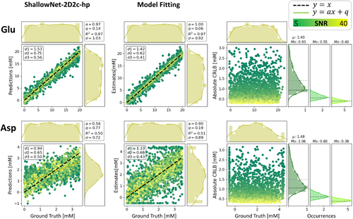
Area-constrained MF shows biases at the parameter boundaries for weakly represented metabolites (e.g., Asp). However, traditional MF outperforms quantification via DL: regression lines show less bias (a and q), and the distribution shape of estimates is closer to a uniform pattern within the GT range. RMSEs (σs) are higher in the case of MF for medium- to weakly represented metabolites (e.g., Asp) but lower for well-defined metabolites (e.g., Glu) (as formerly noted in Figure 7). Consequently, although σs of MF are bigger than the CRLBs estimated for their SNR reference group, σs of DL overestimate CRLBs for well-defined metabolites and underestimate CRLBs for weakly represented metabolites.

4 DISCUSSION

Quantitation of brain metabolites using deep learning methods with spectroscopy data in 1D, 2D, and a combined input format was implemented in multiple network architectures. The main aim of the investigation was to compare the core performance of quantification in an idealized setting of simulated spectra. In fact, the analysis of the optimal performance of both, MF and DL, may otherwise be blurred by additional experimental inaccuracies or artifacts from actual in vitro or in vivo spectra. Moreover, these nuisance contributors may be tackled in separate traditional or DL preprocessing steps that are beyond the current analysis. Many of the methods proved successful in providing absolute concentration values even when using a very large concentration range for the tested metabolites that goes way beyond the near-normal range that has often been used in the past. In addition, different forms of network input were tested, including a specifically tailored time-frequency domain representation and a downscaled water peak for easing of quantification. Whereas data augmentation by active learning schemes showed only modest improvements, ensembles of heterogeneous networks that combine both input representation domains improve the quantitation tasks substantially.

Results from DL predictions were compared to estimates from traditional MF, where it was found that MF is more accurate than DL at high and modest relative noise levels. MF yields higher variance at low SNR, with estimated concentrations artificially aggregated at the boundaries of the fitting parameter range. Predictions obtained with DL algorithms delusively appear more precise (lower RMSE) in the low SNR regime, which may misguide nonexperts to believe that the DL predictions are reliable even at low SNR. However, these predicted concentrations are strongly biased by the dataset the network has been trained with. Hence, in case of high uncertainty (e.g., metabolites with low relative SNR or present in concentrations at the edge of the parameter/training space), the predicted concentration tends toward the most likely value: the average value from the training set.

4.1 Forms of input to networks

Previously, 1D spectra have mostly been used as input for DL algorithms. Here, they have been compared and combined with 2D time-frequency domain spectrograms that had explicitly been designed to be of manageable size while retaining those areas of the high-resolved standard spectrogram that contain the most relevant information, that is, rich in detail in frequency domain to distinguish overlapping spectral features but also maintaining enough temporal structure to characterize ${\mathrm{T}}_2^{\ast }$ signal decay. This comes at the cost that the spectrogram creation cannot be reversed mathematically. However, this is irrelevant when serving as input to a DL network. It was found that this tailored time-frequency representation as input in combination with a shallow CNN architecture performs best and outperforms the use of traditional 1D frequency-domain input for straight quantification or for metabolite basis spectrum isolation with subsequent integration. Furthermore, DL quantitation performance improved upon the inclusion of a downscaled water peak for reference, likely solving scaling issues if no reference is provided.

4.2 Active learning

Active learning has been explored by extending the training dataset with cases that appeared challenging to predict in the original setup. In particular, new training data with nonequal distribution of metabolite concentrations have been used with a predominance of single or multiple metabolites at low or high concentrations. None of these trials led to substantial improvements, although it might be helpful if specific metabolites are targeted primarily. Such data augmentation for all metabolites simultaneously even deteriorated the overall network performance. This can be understood given that augmentation at the border of the concentration range inherently leads to an underrepresentation of intermediate cases, which are equally relevant for the overall performance. Extending the size of the training set even further in an unspecific manner appears to still yield modest improvements.⁷⁵ In addition, an unconventional way of active learning was probed by using unequal dataset ranges in training and testing by limiting testing on the central portion of the training range. This setup clearly ameliorated some of the issues at the edges of the testing range found in the typical setup. This approach was only implemented by reducing the test range rather than expanding the training range, which would yield better comparable outcome scores (e.g., R²). However, expanding the training range to negative concentrations may be questionable.

While data augmentation with a bigger proportion of low SNR spectra leads to worse performance, the theoretical prediction limits for good SNR data are probed in the noiseless scenario in which training and testing are run with GT data. Example results for a ShallowNet architecture are reported in Figure S17 for NAA, GSH, and Lac. This, combined with the results discussed, suggests that the bottleneck that limits higher prediction performances is SNR, just like in traditional MF, regardless of the implementation of state-of-the-art networks, network optimization, or dataset augmentation. It thus reflects limitations in clinical applications where high enough SNR is just not available. According to this study, DL cannot do miracles unless one accepts the bias toward training conditions.⁷³

4.3 Ensemble of networks

An ensemble of networks has been implemented, and it shows improvements for quantifying metabolites. A combination of networks is less sensitive to the specifics of the training and helps reduce the variance in the predictions. Furthermore, ensembles of networks where multiple noise-sensitive predictions are weighted are more robust to noise. However, even the thus optimized networks underperform in comparison to MF. For MF, CRLBs clearly indicate limits for the confidence in the fit results. For DL, including the optimized ensemble of networks, such limits can only vaguely be deduced from the distributions of predicted values with the major danger of bias toward training data norms.^{76, 77} The CRLB would provide good guidance for the valid range of DL predictions as well—although of course they are not readily available without the model. New tools to estimate precision and replace CRLB in the case of DL^{76, 77} still have to prove their value in practice. The situation will be different again if the DL quantification is trained to include cleaning of spectra from artifacts (ghosts, baseline interference) where CRLBs are not available.

4.4 Low SNR regime

Both MF and DL show lower reliability in quantifying metabolites in the low SNR regime. Clear-cut SNR limits for validity of concentration estimates are not available, neither for MF nor for DL, although SNR values are often indicated as measure of spectral quality. While CRLBs provide a widely used and easy-to-interpret reliability measure that includes the influence of SNR, a similar widely accepted concept does currently not extend to DL approaches.⁷⁷ Obviously, a SNR threshold for DL reliability would have to be metabolite-SNR specific, but already the definition of a meaningful metabolite-specific SNR would be cumbersome given that peak-splitting patterns and number of contributing protons as well as lineshape introduce ambiguity. On top, such a metabolite SNR would depend on the estimated metabolite content, whose reliability is at stake. Therefore, just like for MF, global or metabolite-specific SNR will not be informative enough. An uncertainty measure is needed that is based on the predictions and noise distribution but also integrating the uncertainty propagation of the DL model prediction^{78, 79} (like the inverse of the Fisher information matrix used in the CRLB definition⁷⁴). Despite flourishing literature,^{80, 81} addressing uncertainty estimation as a complementary tool for DL interpretability, a full-scale analysis of the robustness and reliability of such models is still challenging.^82-84 First attempts to extend these concepts in DL for MRS quantification are just subject of recent investigations^{76, 77} but far from general acceptance.

4.5 Limitations

The current investigation focused on probing multiple DL techniques and input forms for a full range of metabolite concentrations but a limited range of spectral quality. In particular, the shim remained in a broadly acceptable range, no phase or frequency jitter was considered, and no artifactual data was included. Such features could have been integrated in the current setup to arrive at a more realistic framework. However, the core of the findings (performance of the actual quantification step) is expected to remain in place. In addition, it is recommended to add separate preprocessing steps to prepare the data for the presented algorithms rather than to combine processing and quantification in a single process.³ They could be realized in the form of dedicated DL networks, such as those proposed for phase and frequency drift corrections,^{20, 85, 86} and stacked before the quantification model. This would also ensure the essential gain in speed expected from DL quantification models.

Direct comparison with previously proposed successful DL quantification implementations like Ref. 22 was not possible or meaningful for lack of open access network details and differences in the considered spectra.

Our particular implementation used to create spectrograms was optimized to maintain relevant resolution but downweights the initial part of the FID (initialization of Hamming window). CNN inputs may thus not be fully susceptible to changes in broad signals. Alternative recipes with, for example, prefilled filters or circular datasets, were not explored.

Furthermore, active learning has been explored for a single network type and could in principle be more beneficial for other networks or types of input than what has been found here.

5 CONCLUSIONS

Quantification of MR spectra via diverse and optimized DL algorithms and using 1D and 2D input formats have been explored and have shown adequate performance as long as the metabolite-specific SNR is sufficient. However, as soon as SNR becomes critical, CNN predictions are strongly biased to the training dataset structure.

Traditional MF requires parameter tuning and algorithm convergence, making it more time consuming than DL-based estimates. On the other hand, we have shown that ideally (i.e., with simulated cases) and statistically (i.e., within a variable cohort of cases), it can achieve higher performances when compared to a faster DL approach. DL does not require feature selection by the user, but the potential intrinsic biases at training set boundaries act like soft constraints in traditional modeling,⁹ leading estimated values to the average expected concentration range, which is dangerous in a clinical context that requires the algorithm to be unbiased to outliers (i.e., pathological data).

Active learning and ensemble of networks are attractive strategies to improve prediction performances. However, data quality (i.e., high SNR) has proven as bottleneck for adequate unbiased performance.

ACKNOWLEDGMENTS

This project has received funding from the European Union's Horizon 2020 research and innovation program under the Marie Sklodowska-Curie grant agreement # 813120 (inspire-med) and the Swiss National Science Foundation (#320030-175984). We acknowledge the support of NVIDIA Corporation for the donation of a Titan Xp GPU used for some of this research. The authors thank Prof Maurico Reyes (ARTORG Center for Biomedical Engineering Research, University of Bern, Switzerland) for very helpful discussions.

Open Research

DATA AVAILABILITY STATEMENT

The main part of the code will be available on GitHub (https://github.com/bellarude). In addition, simulated datasets will be available on MRSHub (https://mrshub.org/). For questions, please contact the authors.

Supporting Information

Filename

Description

mrm29561-sup-0001-Supinfo.docxWord 2007 document , 6.7 MB

Table S1. List of probed networks for straight quantification of metabolites and some of their characteristics. The listed characteristics includes the complexity (defined as number of trainable parameters), test loss performance, and training time in sec/epoch. The network identifications were chosen as follows: NetworkType-InputType-properties. 1D: spectra, 2D: spectrograms, 1c: 1 channel, ks3: convolutional kernel size = 3, hp: Bayesian hyper-parameterized architecture, R: exploiting ReLU activations, x2: double convolution before MaxPooling, f: factorized convolution, rb: down-sampling via Reduction-Blocks

Figure S1. Schemes of Residual Network configurations with 1D (a) and 2D (b) inputs, as well as a deep residual network (c). The basic network structure is sketched on the left, the architectures of Residual, Identity, and Convolutional Blocks are reported on the right, while specifications are detailed in the tables in the middle, and symbols are explained near the bottom. The deeper Residual Network configuration has two convolutional layers at the beginning without pooling.

Figure S2. Schemes of Deep CNN configurations with 2D (a) and 1D (b) inputs, as well as an InceptionNet with 1D inputs (c). Network specifications are detailed in the tables, while the architectures of Reduction Blocks are reported on the bottom right. Symbols are explained near the bottom.

Figure S3. Schemes of InceptionNet configurations with 2D inputs on 2 channels. Networks (a) and (b) share the same configuration but (b) exploits convolutional factorization to speed-up training time. (c) Simple concatenation in architectures (a) and (b) are replaced by Reduction Blocks. The architectures of the Reduction Blocks are reported in Figure-S6. Symbols are explained on the right.

Figure S4. Schemes of (a) InceptionNet with 2D inputs and 1 channel, (b) EfficientNetB7, (c) ResNet50 and (d–f) Shallow Network configurations. Networks (a), (b) and (c) are modified from [1–3], respectively. (d) Implements ELU activations, (e) implements RELU activations, whereas (f) implements a deeper configuration with consecutive convolutional layers with sparse pooling. Network specifications are detailed in the tables. Symbols are explained near the bottom.

Figure S5. Scheme and detail of U-Net-1DR-hp configurations for metabolite basis-set prediction. Metabolite-specific network specifications are detailed in the tables. Symbols are explained at the bottom left.

Text S1. Details of Bayesian hyper-parameterization

Figure S6. Examples of dataset augmentation techniques representing sample distributions for two metabolites (NAA and GABA). (a) Dataset size increment with uniform distributed concentrations. (b) and (c) Active Learning weighted on higher occurrences of small and high concentrations for all metabolites in (b) and for selected metabolites in (c). (d) Active Learning weighted on more occurrences of low SNR entries whereas concentration distributions are kept uniform.

Figure S7. Comparison of prediction scores for well-represented and medium-represented metabolites for three CNN architectures with datasets with (red, black, or blue) and without (yellow, gray, or green) water reference. Mean values in orange. On average, water referencing yields higher coefficients a and R² and lower offset q and RMSE σ.

Figure S8. Comparison of prediction scores for medium-represented and weakly-represented metabolites for three CNN architectures with datasets with (red, black, or blue) and without (yellow, gray, or green) water reference. Mean values in orange. On average, water referencing yields higher coefficients a and R² and lower offset q and RMSE σ.

Figure S9. Maps and marginal distributions of predictions vs. GT for a ResNet_1D_hp network. Results for 16 metabolites are arranged in approximate decreasing order of relative SNR from top left to bottom right. RMSE (σ) is reported as an overall measure of variability. A regression model (y = ax + q) is also provided to judge prediction quality. R² measures how well a linear model explains the overall data. Mis-predictions can be monitored either by a decrease in a and R² or by visual biases in distributions of predictions (bell-shape). The prediction bias towards the mean value of the training distribution is evident for medium- to weakly-represented metabolites (e.g., sI, Gly, Asp, PE, Tau, Lac, GABA). On average, metabolites with lower SNR yield higher errors. (q and σ in mM units.).

Figure S10. Maps and marginal distributions of predictions vs. GT for a ShallowNet-2D2c-hp network. Results for 16 metabolites are arranged in approximate decreasing order of relative SNR from top left to bottom right. RMSE (σ) is reported as an overall measure of variability. A regression model (y = ax + q) is also provided to judge prediction quality. R² measures how well a linear model explains the overall data. Mis-predictions can be monitored either by a decrease in a and R² or by visual biases in distributions of predictions (bell-shape). The prediction bias towards the mean value of the training distribution is evident for medium- to weakly-represented metabolites (e.g., sI, Gly, Asp, PE, Tau, Lac, GABA). On average, metabolites with lower SNR yield higher errors. (q and σ in mM units.)

Figure S11. Boxplots comparing the distributions of predictions for 8 metabolites via 7 different CNN architectures vs. Model Fitting estimate distributions (MF) and uniform Ground Truth (GT) distributions. Mis-prediction is evident for medium- to weakly-represented metabolites (e.g., sI, Asp, Tau, Lac) and can be monitored by different degrees of skewness of the boxplot. However, the bias to training distribution is not evident given the visual limitation of boxplots. For better visibility of this outcome, see Figure S14.

Figure S12. Comparison of distributions of predictions for 8 metabolites via 7 different CNN architectures vs. Model Fitting's estimate distributions (MF) and Ground Truth (GT) uniform distributions. Mis-prediction is evident for medium- to weakly-represented metabolites (e.g., sI, Asp, Tau, Lac) and can be monitored by visual biases (bell-shape) towardstoward the mean value of the training distribution (i.e., regression to the mean). Note: y-axes scale inhomogeneously between different networks. However, all distributions integrate to 1.

Figure S13. Concise scores presented to compare quantification quality for different networks and input setups for 16 metabolites. Results reported using the proposed artificial water signal reference. Network identification is chosen as follows: NetworkType-InputType-properties. Keywords: 1D: spectra, 2D: spectrograms, 1c: 1 channel, ks3: convolutional kernel size = 3, hp: Bayesian hyper-parameterized architecture, R: exploiting ReLU activations, x2: double convolution before MaxPooling, f: factorized convolution, rb: down-sampling via Reduction-Blocks.

Figure S14. Comparison of performance scores from different networks for 16 metabolites. Model fitting is included in the comparison.

Text S2. Comparison of predictions from different CNNs.

Figure S15. Comparison of outcomes of Active Learning approaches using concise scores.

Figure S16. Quantification outcome as reflected by concise scores for differently trained single networks and three ensembles of networks (identical training set for 16 metabolites).

Figure S17. Maps and marginal distributions of predictions vs. GT obtained for three metabolites using ShallowNet-2D2c-hp as contrasted for a realistic and noiseless dataset.

Table S2. Results of Active Learning on training set: scores of 16 metabolites for every augmented training set.

Table S3. Results of emulated Active Learning on test set: scores of 16 metabolites for every concentration range considered.

Table S4. Outcome for ensemble learning: scores for 16 metabolites for average network or ensemble of network considered.

Table S5. MRSinMRS checklist.⁸⁷

Please note: The publisher is not responsible for the content or functionality of any supporting information supplied by the authors. Any queries (other than missing content) should be directed to the corresponding author for the article.

REFERENCES

1De Graaf RA. In Vivo NMR Spectroscopy: Principles and Techniques. 3rd ed. John Wiley & Sons; 2019.
10.1002/9781119382461
Google Scholar
2Kreis R, Boer V, Choi IY, et al. Terminology and concepts for the characterization of in vivo MR spectroscopy methods and MR spectra: background and experts' consensus recommendations. NMR Biomed. 2020; 34:e4347. doi:10.1002/nbm.4347
10.1002/nbm.4347
PubMed Web of Science® Google Scholar
3Near J, Harris AD, Juchem C, et al. Preprocessing, analysis and quantification in single-voxel magnetic resonance spectroscopy: experts' consensus recommendations. NMR Biomed. 2021; 34:e4257. doi:10.1002/nbm.4257
10.1002/nbm.4257
PubMed Web of Science® Google Scholar
4Ratiney H, Sdika M, Coenradie Y, Cavassila S, van Ormondt D, Graveron-Demilly D. Time-domain semi-parametric estimation based on a metabolite basis set. NMR Biomed. 2005; 18: 1-13. doi:10.1002/nbm.895
10.1002/nbm.895
CAS PubMed Web of Science® Google Scholar
5Provencher SW. Estimation of metabolite concentrations from localized in vivo proton NMR spectra. Magn Reson Med. 1993; 30: 672-679. doi:10.1002/mrm.1910300604
10.1002/mrm.1910300604
CAS PubMed Web of Science® Google Scholar
6Wilson M, Reynolds G, Kauppinen RA, Arvanitis TN, Peet AC. A constrained least-squares approach to the automated quantitation of in vivo 1H magnetic resonance spectroscopy data. Magn Reson Med. 2011; 65: 1-12. doi:10.1002/mrm.22579
10.1002/mrm.22579
CAS PubMed Web of Science® Google Scholar
7Chong DGQ, Kreis R, Bolliger CS, Boesch C, Slotboom J. Two-dimensional linear-combination model fitting of magnetic resonance spectra to define the macromolecule baseline using FiTAID, a fitting tool for arrays of interrelated datasets. MAGMA. 2011; 24: 147-164. doi:10.1007/s10334-011-0246-y
10.1007/s10334-011-0246-y
PubMed Web of Science® Google Scholar
8Bhogal AA, Schür RR, Houtepen LC, et al. 1H–MRS processing parameters affect metabolite quantification: the urgent need for uniform and transparent standardization. NMR Biomed. 2017; 30:e3804. doi:10.1002/nbm.3804
10.1002/nbm.3804
CAS Web of Science® Google Scholar
9Marjańska M, Deelchand DK, Kreis R, et al. Results and interpretation of a fitting challenge for MR spectroscopy set up by the MRS study group of ISMRM. Magn Reson Med. 2022; 87: 11-32. doi:10.1002/mrm.28942
10.1002/mrm.28942
CAS PubMed Web of Science® Google Scholar
10Lecun Y, Bengio Y, Hinton G. Deep learning. Nature. 2015; 521: 436-444. doi:10.1038/nature14539
10.1038/nature14539
CAS PubMed Web of Science® Google Scholar
11Lundervold AS, Lundervold A. An overview of deep learning in medical imaging focusing on MRI. Z Med Phys. 2019; 29: 102-127. doi:10.1016/j.zemedi.2018.11.002
10.1016/j.zemedi.2018.11.002
PubMed Web of Science® Google Scholar
12Lam F, Li Y, Peng X. Constrained magnetic resonance spectroscopic imaging by learning nonlinear low-dimensional models. IEEE Trans Med Imaging. 2020; 39: 545-555. doi:10.1109/TMI.2019.2930586
10.1109/TMI.2019.2930586
PubMed Web of Science® Google Scholar
13Klukowski P, Augoff M, ZieRba M, Drwal M, Gonczarek A, Walczak MJ. NMRNet: a deep learning approach to automated peak picking of protein NMR spectra. Bioinformatics. 2018; 34: 2590-1597. doi:10.1093/bioinformatics/bty134
10.1093/bioinformatics/bty134
CAS PubMed Web of Science® Google Scholar
14Hatami N, Sdika M, Ratiney H. Magnetic resonance spectroscopy quantification using deep learning. Lect Notes Comput Sci. 2018; 11070: 467-475. doi:10.1007/978-3-030-00928-1_53
10.1007/978?3?030?00928?1_53
Google Scholar
15Lee H, Lee HH, Kim H. Reconstruction of spectra from truncated free induction decays by deep learning in proton magnetic resonance spectroscopy. Magn Reson Med. 2020; 84: 559-568. doi:10.1002/mrm.28164
10.1002/mrm.28164
CAS PubMed Web of Science® Google Scholar
16Iqbal Z, Nguyen D, Thomas MA, Jiang S. Deep learning can accelerate and quantify simulated localized correlated spectroscopy. Sci Rep. 2021; 11: 8727. doi:10.1038/s41598-021-88158-y
10.1038/s41598?021?88158?y
CAS PubMed Web of Science® Google Scholar
17Lee HH, Kim H. Intact metabolite spectrum mining by deep learning in proton magnetic resonance spectroscopy of the brain. Magn Reson Med. 2019; 82: 33-48. doi:10.1002/mrm.27727
10.1002/mrm.27727
CAS PubMed Web of Science® Google Scholar
18Kyathanahally SP, Döring A, Kreis R. Deep learning approaches for detection and removal of ghosting artifacts in MR spectroscopy. Magn Reson Med. 2018; 80: 851-863. doi:10.1002/mrm.27096
10.1002/mrm.27096
PubMed Web of Science® Google Scholar
19Gurbani SS, Schreibmann E, Maudsley AA, et al. A convolutional neural network to filter artifacts in spectroscopic MRI. Magn Reson Med. 2018; 80: 1765-1775. doi:10.1002/mrm.27166
10.1002/mrm.27166
PubMed Web of Science® Google Scholar
20Tapper S, Mikkelsen M, Dewey BE, et al. Frequency and phase correction of J-difference edited MR spectra using deep learning. Magn Reson Med. 2021; 85: 1755-1765. doi:10.1002/mrm.28525
10.1002/mrm.28525
PubMed Web of Science® Google Scholar
21Jang J, Lee HH, Park JA, Kim H. Unsupervised anomaly detection using generative adversarial networks in 1H-MRS of the brain. J Magn Reson. 2021; 325:106936. doi:10.1016/j.jmr.2021.106936
10.1016/j.jmr.2021.106936
CAS PubMed Web of Science® Google Scholar
22Lee HH, Kim H. Deep learning-based target metabolite isolation and big data-driven measurement uncertainty estimation in proton magnetic resonance spectroscopy of the brain. Magn Reson Med. 2020; 84: 1689-1706. doi:10.1002/MRM.28234
10.1002/MRM.28234
CAS PubMed Web of Science® Google Scholar
23Gurbani SS, Sheriff S, Maudsley AA, Shim H, Cooper LAD. Incorporation of a spectral model in a convolutional neural network for accelerated spectral fitting. Magn Reson Med. 2019; 81: 3346-3357. doi:10.1002/mrm.27641
10.1002/mrm.27641
PubMed Web of Science® Google Scholar
24Chandler M, Jenkins C, Shermer SM, Langbein FC. MRSNet: metabolite quantification from edited magnetic resonance spectra with convolutional neural networks. 2019 arXiv:1909.03836v1 [eess.IV]. 10.48550/arXiv.1909.03836
Google Scholar
25Litjens G, Kooi T, Bejnordi BE, et al. A survey on deep learning in medical image analysis. Med Image Anal. 2017; 42: 60-88. doi:10.1016/J.MEDIA.2017.07.005
10.1016/j.media.2017.07.005
PubMed Web of Science® Google Scholar
26Gyori NG, Palombo M, Clark CA, Zhang H, Alexander DC. Training data distribution significantly impacts the estimation of tissue microstructure with machine learning. Magn Reson Med. 2022; 87: 932-947. doi:10.1002/MRM.29014
10.1002/MRM.29014
PubMed Web of Science® Google Scholar
27Espi M, Fujimoto M, Kinoshita K, Nakatani T. Exploiting spectro-temporal locality in deep learning based acoustic event detection. J Audio Speech Music Proc. 2015; 2015: 26. doi:10.1186/s13636-015-0069-2
10.1186/s13636?015?0069?2
Google Scholar
28Thomas S, Ganapathy S, Saon G, Soltau H. Analyzing convolutional neural networks for speech activity detection in mismatched acoustic conditions. In 2014 IEEE International Conference on Acoustics, Speech and Signal Processing (ICASSP); 2014: 2519–2523. 10.1109/ICASSP.2014.6854054
Google Scholar
29Alaskar H. Deep learning-based model architecture for time-frequency images analysis. Int J Adv Comput Sci Appl. 2018; 9: 486-494. doi:10.14569/IJACSA.2018.091268
10.14569/IJACSA.2018.091268
Web of Science® Google Scholar
30Zagoruyko S, Komodakis N. Wide residual networks. In ArXiv; 2017:arXiv:1605.07146. 10.5244/C.30.87
Google Scholar
31Cohn DA, Ghahramani Z, Jordan MI. Active learning with statistical models. J Artif Intell Res. 1996; 4: 129-145. doi:10.1613/JAIR.295
10.1613/JAIR.295
Web of Science® Google Scholar
32Hansen LK, Salamon P. Neural network ensembles. IEEE Trans Pattern Anal Mach Intell. 1990; 12: 993-1001. doi:10.1109/34.58871
10.1109/34.58871
Web of Science® Google Scholar
33Krizhevsky A, Sutskever I, Hinton GE. ImageNet classification with deep convolutional neural networks. Commun ACM. 2017; 60: 84-90. doi:10.1145/3065386
10.1145/3065386
Web of Science® Google Scholar
34Patra S, Bruzzone L. A cluster-assumption based batch mode active learning technique. Pattern Recognit Lett. 2012; 33: 1042-1048. doi:10.1016/J.PATREC.2012.01.015
10.1016/J.PATREC.2012.01.015
Web of Science® Google Scholar
35Maiora J, Ayerdi B, Graña M. Random forest active learning for AAA thrombus segmentation in computed tomography angiography images. Neurocomputing. 2014; 126: 71-77. doi:10.1016/J.NEUCOM.2013.01.051
10.1016/J.NEUCOM.2013.01.051
Web of Science® Google Scholar
36Kutsuna N, Higaki T, Matsunaga S, et al. Active learning framework with iterative clustering for bioimage classification. Nat Commun. 2012; 3: 1032. doi:10.1038/ncomms2030
10.1038/ncomms2030
PubMed Web of Science® Google Scholar
37Lewis DD, Gale WA. A sequential algorithm for training text classifiers. In the 17th Annual International ACM SIGIR Conference on Research and Development in Information Retrieval, 1994: 3–12. 10.1007/978-1-4471-2099-5_1
Google Scholar
38Tuia D, Ratle F, Pacifici F, Kanevski MF, Emery WJ. Active learning methods for remote sensing image classification. IEEE Trans Geosci Remote Sens. 2009; 48: 2218-2232. doi:10.1109/TGRS.2008.2010404
10.1109/TGRS.2008.2010404
Web of Science® Google Scholar
39Silva C, Ribeiro B. Margin-based active learning and background knowledge in text mining. In the 4th International Conference on Hybrid Intelligent Systems, 2005: 8–13. 10.1109/ICHIS.2004.70
Google Scholar
40Pedrosa de Barros N, McKinley R, Wiest R, Slotboom J. Improving labeling efficiency in automatic quality control of MRSI data. Magn Reson Med. 2017; 78: 2399-2405. doi:10.1002/mrm.26618
10.1002/mrm.26618
CAS PubMed Web of Science® Google Scholar
41Bishop CM. Neural Networks for Pattern Recognition. Oxford University Press; 2005.
Google Scholar
42Freund Y, Schapire RE. A decision-theoretic generalization of on-line learning and an application to boosting. J Comput Syst Sci. 1997; 55: 119-139. doi:10.1006/jcss.1997.1504
10.1006/jcss.1997.1504
Web of Science® Google Scholar
43Chen T, Guestrin C. XGBoost: a scalable tree boosting system. In the 22nd International Conference on Knowledge Discovery and Data Mining; 2016: 785–794. 10.1145/2939672
Google Scholar
44Ke G, Meng Q, Finley T, et al. LightGBM: a highly efficient gradient boosting decision tree. In the 31st International Conference on Neural Information Processing Systems; 2017: 3149–3157. 10.5555/3294996
Google Scholar
45Soher BJ, Semanchuk P, Todd D, Steinberg J, Young K. VeSPA: integrated applications for RF pulse design, spectral simulation and MRS data analysis. In Proceedings of the 19th Annual Meeting of ISMRM, Montréal, Québec, Canada. 2011, 1410.
Google Scholar
46Oz G, Tkac I. Short-echo, single-shot, full-intensity proton magnetic resonance spectroscopy for neurochemical profiling at 4 T: validation in the cerebellum and brainstem. Magn Reson Med. 2011; 65: 901-910. doi:10.1002/mrm.22708
10.1002/mrm.22708
CAS PubMed Web of Science® Google Scholar
47 The Mathworks Inc. MATLAB (R2019a).MathWorks Inc 2019.
Google Scholar
48Marjańska M, McCarten JR, Hodges J, et al. Region-specific aging of the human brain as evidenced by neurochemical profiles measured noninvasively in the posterior cingulate cortex and the occipital lobe using 1H magnetic resonance spectroscopy at 7 T. Neuroscience. 2017; 354: 168-177. doi:10.1016/j.neuroscience.2017.04.035
10.1016/j.neuroscience.2017.04.035
CAS PubMed Web of Science® Google Scholar
49Hoefemann M, Bolliger CS, Chong DGQ, van der Veen JW, Kreis R. Parameterization of metabolite and macromolecule contributions in interrelated MR spectra of human brain using multidimensional modeling. NMR Biomed. 2020; 33:e4328. doi:10.1002/nbm.4328
10.1002/nbm.4328
CAS PubMed Web of Science® Google Scholar
50Bottomley PA, Griffiths JR. Handbook of Magnetic Resonance Spectroscopy in Vivo: MRS Theory, Practice and Applications. 1st ed. Hoboken, NJ, Wiley & Sons; 2016.
Google Scholar
51Oz G, Alger JR, Barker PB, et al. Clinical proton MR spectroscopy in central nervous system disorders. Radiology. 2014; 270: 658-679.
10.1148/radiol.13130531
PubMed Web of Science® Google Scholar
52Träber F, Block W, Lamerichs R, Gieseke J, Schild HH. 1H metabolite relaxation times at 3.0 Tesla: measurements of T1 and T2 values in normal brain and determination of regional differences in transverse relaxation. J Magn Reson Imaging. 2004; 19: 537-545. doi:10.1002/jmri.20053
10.1002/jmri.20053
CAS PubMed Web of Science® Google Scholar
53An L, Li S, Shen J. Simultaneous determination of metabolite concentrations, T1 and T2 relaxation times. Magn Reson Med. 2017; 78: 2072-2081.
10.1002/mrm.26612
CAS PubMed Web of Science® Google Scholar
54Zhang Y, Shen J. Simultaneous quantification of glutamate and glutamine by J-modulated spectroscopy at 3 Tesla. Magn Reson Med. 2016; 76: 725-732.
10.1002/mrm.25922
CAS PubMed Web of Science® Google Scholar
55Cudalbu C, Behar KL, Bhattacharyya PK, et al. Contribution of macromolecules to brain 1H MR spectra: experts' consensus recommendations. NMR Biomed. 2021; 34:e4393. doi:10.1002/nbm.4393
10.1002/nbm.4393
PubMed Web of Science® Google Scholar
56Van RG, Drake FL. Python 3 Reference Manual. CreateSpace; 2009.
Google Scholar
57Gulli A, Pal S. Deep Learning with Keras. Packt Publishing; 2017.
Google Scholar
58Abadi M, Barham P, Chen J, et al. TensorFlow: a system for large-scale machine learning. In the 12th USENIX Symposium on Operating Systems Design and Implementation; 2016: 265–283. 10.5555/3026877.3026899
Google Scholar
59Bisong E. Google colaboratory. Building Machine Learning and Deep Learning Models on Google Cloud Platform. Apress, New York City; 2019. doi:10.1007/978-1-4842-4470-8_7
10.1007/978?1?4842?4470?8_7
Google Scholar
60Simonyan K, Zisserman A. Very deep convolutional networks for large-scale image recognition. In arXiv; 2015:1409.1556.
Google Scholar
61He K, Zhang X, Ren S, Sun J. Deep residual learning for image recognition. In the 2016 IEEE Computer Society Conference on Computer Vision and Pattern Recognition (CVPR); 2016: 770–778. 10.1109/CVPR.2016.90
Google Scholar
62Szegedy C, Vanhoucke V, Ioffe S, Shlens J, Wojna Z. Rethinking the inception architecture for computer vision. In the 2016 IEEE Computer Society Conference on Computer Vision and Pattern Recognition (CVPR); 2016: 2818–2826. 10.1109/CVPR.2016.308
Google Scholar
63Szegedy C, Liu W, Jia Y, et al. Going deeper with convolutions. In 2015 IEEE Computer Society Conference on Computer Vision and Pattern Recognition (CVPR); 2015: 1–9. 10.1109/CVPR.2015.7298594
Google Scholar
64Szegedy C, Ioffe S, Vanhoucke V, Alemi AA. Inception-v4, inception-ResNet and the impact of residual connections on learning. In the 31st AAAI Conference on Artificial Intelligence; 2017: 4278–4284. 10.48550/arXiv.1602.07261
Google Scholar
65Ioffe S, Szegedy C. Batch normalization: accelerating deep network training by reducing internal covariate shift. In ArXiv; 2015:arXiv:1502.03167.
Google Scholar
66Clevert DA, Unterthiner T, Hochreiter S. Fast and accurate deep network learning by exponential linear units (ELUs). In: ArXiv; 2016:arXiv:1511.07289.
Google Scholar
67Snoek J, Larochelle H, Adams RP. Practical Bayesian optimization of machine learning algorithms. In: ArXiv; 2012:arXiv:1206.2944.
Google Scholar
68Rizzo R, Kreis R. Accounting for bias in estimated metabolite concentrations from cohort studies as caused by limiting the fitting parameter space. In Proceedings of the 2021 ISMRM & SMRT Annual Meeting and Exhibition, Virtual meeting, May 15–20, 2021. p. 2011.
Google Scholar
69Ronneberger O, Fischer P, Brox T. U-Net: convolutional networks for biomedical image segmentation. Lect Notes Comput Sci. 2015; 9351: 234-241. doi:10.1007/978-3-319-24574-4_28
10.1007/978-3-319-24574-4_28
Google Scholar
70Kingma DP, Ba JL. Adam: a method for stochastic optimization. In ArXiv; 2017:arXiv:1412.6980.
Google Scholar
71Bengio Y. Practical recommendations for gradient-based training of deep architectures. Lect Notes Comput Sci. 2012; 7700: 437-478.
10.1007/978-3-642-35289-8_26
Google Scholar
72Bengio Y, Goodfellow IJ, Courville A. Optimization for training deep models. Deep Learning. MIT Press; 2016.
Google Scholar
73Landheer K, Juchem C. Are Cramér-Rao lower bounds an accurate estimate for standard deviations in in vivo magnetic resonance spectroscopy? NMR Biomed. 2021; 34:e4521. doi:10.1002/nbm.4521
10.1002/nbm.4521
CAS PubMed Web of Science® Google Scholar
74Bolliger CS, Boesch C, Kreis R. On the use of Cramér-Rao minimum variance bounds for the design of magnetic resonance spectroscopy experiments. Neuroimage. 2013; 83: 1031-1040. doi:10.1016/j.neuroimage.2013.07.062
10.1016/j.neuroimage.2013.07.062
PubMed Web of Science® Google Scholar
75Hong S, Shen J. Impact of training size on deep learning performance in in vivo 1H MRS. In Proceedings of the 2021 ISMRM & SMRT Annual Meeting and Exhibition, Virtual meeting, May 15–20, 2021, p. 2015.
Google Scholar
76Lee HH, Kim H. Bayesian deep learning-based 1 H-MRS of the brain: metabolite quantification with uncertainty estimation using Monte Carlo dropout. Magn Reson Med. 2022; 88: 38-52. doi:10.1002/MRM.29214
10.1002/MRM.29214
PubMed Web of Science® Google Scholar
77Rizzo R, Dziadosz M, Kyathanahally SP, Reyes M, Kreis R. Reliability of quantification estimates in MR spectroscopy: CNNs vs traditional model fitting. Med Image Comput Comput Assist Interv–MICCAI 2022 Lect Notes Comput Sci. 2022; 13438: 715-724. doi:10.1007/978-3-031-16452-1_68
10.1007/978?3?031?16452?1_68
Google Scholar
78Gal Y. 2016 Uncertainty in deep learning. https://mlg.eng.cam.ac.uk/yarin/thesis/thesis.pdf
Google Scholar
79Kendall A, Gal Y. What uncertainties do we need in Bayesian deep learning for computer vision? In the 31st Conference on Neural Information Processing Systems (NIPS); 2017.
Google Scholar
80Sanchez T, Caramiaux B, Thiel P, Mackay WE. Deep learning uncertainty in machine teaching. In 27th Annual Conference on Intelligent User Interfaces (IUI), Vol. 1, 2022. 10.1145/3490099.3511117
Google Scholar
81Abdar M, Pourpanah F, Hussain S, et al. A review of uncertainty quantification in deep learning: techniques, applications and challenges. Inf Fusion. 2021; 76: 243-297. doi:10.1016/j.inffus.2021.05.008
10.1016/j.inffus.2021.05.008
Web of Science® Google Scholar
82Jungo A, Reyes M. Assessing reliability and challenges of uncertainty estimations for medical image segmentation. In International Conference on Medical Image Computing and Computer Assisted Intervention – MICCAI 2019: 22nd International Conference, Proceedings, Part II. Berlin, Heidelberg, Springer-Verlag. 10.1007/978-3-030-32245-8_6
Google Scholar
83Ennab M, McHeick H. Designing an interpretability-based model to explain the artificial intelligence algorithms in healthcare. Diagnostics. 2022; 12: 1557. doi:10.3390/DIAGNOSTICS12071557
10.3390/DIAGNOSTICS12071557
PubMed Web of Science® Google Scholar
84Meng C, Trinh L, Xu N, Enouen J, Liu Y. Interpretability and fairness evaluation of deep learning models on MIMIC-IV dataset. Sci Rep. 2022; 12: 1-28. doi:10.1038/s41598-022-11012-2
10.1038/s41598?022?11012?2
PubMed Web of Science® Google Scholar
85Ma DJ, Le HAM, Ye Y, et al. MR spectroscopy frequency and phase correction using convolutional neural networks. Magn Reson Med. 2022; 87: 1700-1710. doi:10.1002/MRM.29103
10.1002/MRM.29103
PubMed Web of Science® Google Scholar
86 Shamaei AM, Starcukova J, Pavlova I, Starcuk Z. Model-informed unsupervised deep learning approaches to frequency and phase correction of MRS signals. bioRxiv. 2022. doi:10.1101/2022.06.28.497332
10.1101/2022.06.28.497332
Google Scholar
87Lin A, Andronesi O, Bogner W, et al. Minimum reporting standards for in vivo magnetic resonance spectroscopy (MRSinMRS): Experts' consensus recommendations. NMR Biomed. 2021; 34:e4484. doi:10.1002/nbm.4484
10.1002/nbm.4484
PubMed Web of Science® Google Scholar

Citing Literature

Volume89, Issue5

May 2023

Pages 1707-1727

Quantification of MR spectra by deep learning in an idealized setting: Investigation of forms of input, network architectures, optimization by ensembles of networks, and training bias

Abstract

Purpose

Methods

Results

Conclusion

1 INTRODUCTION

2 METHODS

2.1 Simulations

2.1.1 MR spectra

2.1.2 Spectrograms

2.2 Design and training of CNN architectures

2.2.1 Architectures for straight numeric quantification of concentrations

2.2.2 Architectures for estimation of metabolite base spectra

2.2.3 Training

2.2.4 Evaluation

2.3 Influence of inclusion of water reference peak

2.4 Active learning and dataset size

2.5 Ensemble of networks

2.6 Model fitting

3 RESULTS

3.1 S1Metabolite quantification referenced to the downscaled water peak

3.2 Network design

3.3 Dataset size, active learning, and ensembles of networks

3.3.1 Dataset size

3.3.2 Active learning

3.3.3 Ensemble of networks

3.4 CNN predictions versus model fitting estimates

4 DISCUSSION

4.1 Forms of input to networks

4.2 Active learning

4.3 Ensemble of networks

4.4 Low SNR regime

4.5 Limitations

5 CONCLUSIONS

ACKNOWLEDGMENTS

Open Research

DATA AVAILABILITY STATEMENT

Supporting Information

REFERENCES

Citing Literature

Figures

References

Related

Information