Rapid estimation of 2D relative -maps from localizers in the human heart at 7T using deep learning
Click here for author-reader discussions
Parts of this work have been presented at the 2022 Annual Meeting of the International Society for Magnetic Resonance in Medicine.
Funding information: German Research Foundation, Grant/Award Numbers: SCHM 2677/2-1; SCHM 2677/4-1; GRK2260-BIOQIC
Abstract
Purpose
Subject-tailored parallel transmission pulses for ultra-high fields body applications are typically calculated based on subject-specific -maps of all transmit channels, which require lengthy adjustment times. This study investigates the feasibility of using deep learning to estimate complex, channel-wise, relative 2D -maps from a single gradient echo localizer to overcome long calibration times.
Methods
126 channel-wise, complex, relative 2D -maps of the human heart from 44 subjects were acquired at 7T using a Cartesian, cardiac gradient-echo sequence obtained under breath-hold to create a library for network training and cross-validation. The deep learning predicted maps were qualitatively compared to the ground truth. Phase-only -shimming was subsequently performed on the estimated -maps for a region of interest covering the heart. The proposed network was applied at 7T to 3 unseen test subjects.
Results
The deep learning-based -maps, derived in approximately 0.2 seconds, match the ground truth for the magnitude and phase. The static, phase-only pulse design performs best when maximizing the mean transmission efficiency. In-vivo application of the proposed network to unseen subjects demonstrates the feasibility of this approach: the network yields predicted -maps comparable to the acquired ground truth and anatomical scans reflect the resulting -pattern using the deep learning-based maps.
Conclusion
The feasibility of estimating 2D relative -maps from initial localizer scans of the human heart at 7T using deep learning is successfully demonstrated. Because the technique requires only sub-seconds to derive channel-wise -maps, it offers high potential for advancing clinical body imaging at ultra-high fields.
1 INTRODUCTION
Magnetic resonance imaging (MRI) at ultra-high fields (UHF) provides ample opportunities for imaging the human body because of an intrinsic gain in signal-to-noise ratio (SNR), a higher chemical shift, and in many cases, a stronger contrast.1 However, the shortened radiofrequency (RF) wavelength within the tissue at 7T and the resulting constructive and destructive interference of the transmit (Tx) magnetic fields () can lead to spatially nonuniform distributions of the flip angle (FA) and contrast, as well as to local signal dropouts.2 Such effects reduce the diagnostic value of UHF MRI3 when relying on conventional single-channel transmission imaging, especially when targeting the human body.
Parallel transmission (pTx) in combination with multi-Tx coils allows to spatially shape the amplitude and phase of -distributions in the human body2, 4-7 using dedicated RF pulses. Such pTx methods can be divided into (1) calibration-free methods, which do not require additional calibration before the actual measurement, and (2) subject-tailored approaches.
A straight forward calibration-free pTx technique would be to drive all Tx channels with a fixed -phase (amplitude) setting for all subjects. The used shim vector is often calculated from electromagnetic simulations for a given target volume.8, 9 To reduce remaining contrast variations, the TIAMO method10 acquires multiple scans with different shim settings at the cost of doubling the acquisition time. The application of pre-computed universal pulses, originally developed for the human head,11 is a data-driven, calibration-free method and it has been recently demonstrated in the body at 7T.12 Universal pulses and fixed -phase approaches typically come at the expense of reduced FA homogeneity as compared to subject-tailored solutions that optimize pulses for every individual subject.11-13
Subject-tailored pTx pulses are typically calculated based on subject-specific -maps of all Tx channels, which require potentially lengthy adjustment times at the beginning of the study. Although rapid 3D -mapping of the entire brain at 7T can be achieved within only 40 seconds or less for 8 Tx channels,13 the acquisition in the body is challenging. Scan times in the thorax can be substantially longer because of the larger field of view (FOV) and different sources of motion.14 Furthermore, some of the faster techniques applied to the brain, such as DREAM15 or Bloch-Siegert based mapping,16 cannot be transferred straightforwardly to the body because of the sensitivity to blood flow or high RF power levels required at 7T, therefore, leaving only a few options for -mapping in the human body. Several works have used -mapping methods in a slice-selective manner to limit scan times to acquire the data within a breath-hold of fewer than 20 seconds.10, 15, 17, 18 However, when FA optimization over a 3D volume is desired, multi-slice 2D or 3D -maps with scan times of more than 3 minutes19 need to be acquired, requiring multiple breath-hold scans or free respiratory navigation. Recent preliminary work showed fast -mapping based on pre-saturated TurboFLASH sequences20-22 in under a minute. However, reconstruction times of at least 8 minutes were needed. In addition to the time required for mapping and reconstructing , further calibration time is necessary for the RF pulse calculation, which depends on the complexity of the desired FA pattern. In total, an overall calibration time of more than 10 minutes is not uncommon for the human body in practice, which is one of the major drawbacks of UHF body MRI in clinical applications.
In recent works, deep learning (DL) techniques have shown promising results in reducing the RF pulse calculation times.23-25 Vinding et al.23 proposed a DL-based RF pulse design for high-FA 2D RF pulses at 7T with a pulse prediction time of under 10 milliseconds. Furthermore, different neural networks have been suggested to approximate channel-combined or channel-wise -distributions in various application scenarios.25-29 Abbasi-Rad et al.28 reduced the specific absorption rate (SAR) in T2-FLAIR imaging at UHF in the human head by determining a scaling factor for adiabatic RF pulses from a predicted channel-combined -magnitude. Plumley et al.29 presented a system of conditional generative adversarial networks to predict how rigid motion changes complex, channel-wise -distributions in the head. This framework is highly suited for real-time pTx pulse re-design, but requires the initial channel-wise -maps. Eberhardt et al.25 used -maps of only some of the 16 Tx channels of a 7T head coil and applied image-to-image translation networks to augment the data to a complete set of channel-wise -maps in the head. This approach achieved comparable FA homogenization results to those obtained from a full calibration data set if half of the Tx-channel-wise -maps were acquired.25 Nevertheless, the need to substantially reduce the calibration time in the human body at 7T to a duration comparable to typical adjustment times of clinical scans of a few seconds remains unanswered. Yet, all recent DL techniques focused on the human brain or still needed a significant amount of input information.
In this proof-of-concept study, we reduce the time to obtain subject-specific -maps for subject-tailored cardiac pTx at 7T to a minimum. This is achieved by deriving complex, relative, channel-wise 2D -maps of 8 Tx channels from a single gradient-echo (GRE) localizer scan obtained in a combined 1-Tx mode with 32 receive (Rx) channels using DL. Because such localizer scans are acquired anyway for planning at the beginning of the session, this approach does not add any additional scan time for -mapping. -phase shimming vectors are calculated based on the estimated -maps for a region of interest (ROI) covering the heart, and the predicted (PR) channel-wise -maps and resulting shimmed -fields are tested against the ground truth (GT). Finally, the feasibility of this approach is demonstrated in vivo.
2 METHODS
The proposed method of this work is to replace the -mapping step for subject-tailored pTx at 7T by a DL estimation approach. The neural network was trained on acquired localizer data serving as input and the corresponding -maps as GT. The performance of the network was assessed by calculating -phase shimming vectors based on the PR data and by an in-vivo application.
2.1 Hardware and setups
All data were acquired on a 7T whole-body MRI scanner (Magnetom 7T, Siemens, Erlangen, Germany) with an 8-channel transmit array and a whole-body gradient system using a commercial 32-element (8 dipoles and 24 loops) body coil array (MRI.TOOLS, Berlin, Germany). The coil comprised of two halves, a posterior and an anterior, each containing 16 elements. In the transmit case, the 32 elements were driven in an 8 Tx mode, in which four elements (1 dipole and 3 loops arranged along the dipole) were combined with hardware-fixed RF phases. In the receive case, all 32 elements operated independently using the 32 Rx channels of the system. The subjects were scanned in a supine position with the heart in the isocenter.
Reconstruction of the complex localizer data, manual selection of 2D heart and thorax ROIs, and static pulse design was carried out on a separate workstation (12 cores with 2.1 GHz, 128 GB RAM) using a custom-built toolbox written in MATLAB (Version 2020a, The MathWorks, Natick, MA, USA). The prediction of the relative -maps using the suggested neural network was executed within the Google Colab environment (Google LLC, Mountain View, CA, USA).
2.2 Data acquisition and processing
For the proposed neural network, 2 libraries containing complex localizers as input and channel-wise -maps as GT (Figure 1A) of healthy subjects were included in this study following approval of an internal review board and after written and informed consent. A performance library used for cross-validation comprised of 44 subjects (age: 34 ± 11 years, max/min: 66/21 years; body mass index (BMI): 23.79 kg/m2 ± 3.10 kg/m2, max/min: 34/19 kg/m2, skewness: 0.96; male/female: 27/17), whereas an application library was used for in-vivo application.
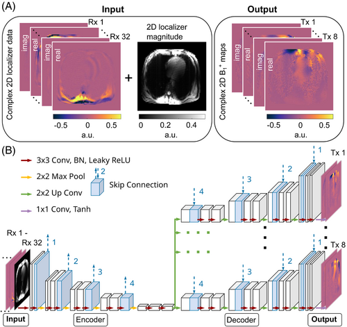
For the input of the neural network, a GRE localizer was acquired with all Tx channels transmitting with the default phase setting (i.e., an RF phase optimized by the vendor based on electromagnetic simulations for the heart and aorta). However, the performance of this default setting depends on the size and shape of the human body and may yield destructive interferences in the heart.6 The parameters for this protocol were as follows: nominal , , , , , resolution , slice thickness , slice distances , flow compensation along slice/readout direction, no parallel imaging, no partial Fourier applied.
Subsequently, the same acquisition was repeated eight times using identical parameters with only a single Tx channel active per measurement. The active channel was incremented across scans. Following the approach by van de Moortele et al.,19, 30 channel-wise, relative 2D -maps (i.e., an absolute scaling factor of the maps was unknown) were calculated using these eight measurements. These maps served as the neural network's GT. Although this fast technique provides only relative -maps, it has been demonstrated to be highly suited for multiple body applications in UHF imaging, including static7 and dynamic pTx for cardiac MRI.6, 31, 32 Unlike in previous works,6, 32, 33 the phase distributions were not calculated relative to one channel, but instead relative to the phase of the superimposed complex data of transmit channels 2, 3, and 4, which are located posterior and anterior to the subject. This resulted in a sufficient -magnitude in the heart for the reference signal, ensuring smooth, complex-valued data. The nine GRE acquisitions (one localizer and eight for -mapping) were obtained transversal in all subjects for 3 slice locations with 20 mm distance. In some subjects, the top or bottom slice contained only a small section of the apex or atria. For four subjects, one affected slice was not included in the final data set. Only one slice was available in one case. As a result, the performance library for cross-validation of the neural network comprised 126 slices, including the complex, 2D localizer data from 32 Rx channels and relative, channel-wise, 2D -maps from 8 Tx channels (Figure 1A).
The data were pre-processed as follows: real and imaginary parts of the 32 Rx-channel-wise localizers and 8 calculated Tx-channel-wise -maps were separated. Normalization by the maximum absolute value of the complex localizer for the input and the maximum absolute value of the complex -distribution for the GT was conducted to ensure a comparable dynamic range in the complex data across different subjects between 0 and 1. The 32 Rx-channel-wise localizer slices in the image domain were used as input for the network leading to an overall input size of 96 × 96 × 65, i.e., the 32 real, 32 imaginary Rx-channel-wise localizers, and one magnitude image using the root-sum-of-squares across all Rx channels.
Correspondingly, the 8 Tx-channel-wise -maps resulted in a size of 96 × 96 × 16 serving as GT. The sum-of-magnitudes (SOM) of the -maps were used to manually select a binary mask (ROI1) covering the thorax for every slice and subject. This mask was then multiplied pixel-wise with the input and output data to suppress the noise signal outside the thorax. This step was repeated for another mask (ROI2) covering the heart to be used for static pulse design and quantitative evaluation.
2.3 Network architecture and model evaluation
The proposed neural network was based on a modified version of the established 2D UNet architecture34, 35 to predict complex, Tx-channel-wise, 2D -maps from complex, Rx-channel-wise 2D localizer data (Figure 1B). This architecture is suitable for a plethora of applications, for example, image reconstruction,36, 37 quantitative parameter mapping,38, 39 and artifact correction.37, 40 The chosen architecture comprised four encoding stages, each including a 2 × 2 max pooling layer (downsampling) and 2 repetitions of 3 × 3 convolutions, batch normalizations, and LeakyReLU activation functions. For decoding, the structure was split into eight parallel pipelines, with one output -map for each Tx channel connecting the 32-Rx-channel localizer input data with an overall input size of 96 × 96 × 65 with the corresponding 8 Tx channel -maps with an overall size of 96 × 96 × 16. Each decoder stage included a 2 × 2 up convolution layer (upsampling), 2 repetitions of 3 × 3 convolutions, batch normalizations, and LeakyReLU activation functions. The number of output filters was set to 32 in the first and last layer and was doubled/halved per encoding/decoding stage, up to a maximum of 512 filters. The network used skip connections between corresponding stages to reduce spatial resolution losses and avoid vanishing gradients.41 To minimize overfitting, dropout layers were used for regularization with an increasing dropout rate per stage.
The minimization was conducted using the ADAM optimizer. For better convergence, a decaying learning rate44 was used: for the j-th epoch to achieve a decrease in the learning rate of one magnitude after 4000 epochs. The model was trained for 4000 epochs with a batch size of 2, leading to a training time of approximately 240 min. The code for implementing the neural network, the network weights, the data libraries, and pulse design and analysis algorithms can be downloaded from https://github.com/felixkrueger90/DeepB1.
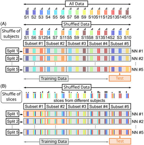
The quality of the PR -maps (i.e., its resemblance to the GT) was evaluated via image quality metrics assessed through the root-mean-squared error (RMSE) and structural similarity index measure (SSIM) performed on the ROI1-masked thorax data. A 5-fold cross-validation was carried out on the entirety of the performance library (Figure 2A) to evaluate the model's generalization performance on all thorax geometries. First, all data were randomly shuffled at the subject level and split into 5 subsets containing 8/9 subjects each. Therefore, every subject is included in only one of the subsets. One subset is kept as unseen test data, and the other 4 are used for network training. This process was repeated five times, with each subset being the test data once. For every data split, approximately 20% of all 44 subjects (8/9 subjects) were used for testing and 80% (35/36 subjects) for training.
2.4 Pulse design and analysis
To access the quality of the PR -maps and the feasibility of the approach in context of a subject-specific calibration, the -shim vectors bHom, bEff, and bEnf were calculated based on the PR -maps. The shim vectors were then applied to both the PR and GT -maps to generate the combined -map when all Tx channels transmit together. These combined maps based on the GT and PR were quantitatively compared for all three settings and the default shim bDef in terms of CV and mean efficiency optimized for ROI2 covering the heart.
2.5 Experimental application
The application library was acquired for in-vivo application of the proposed approach. The library contained three subjects (1 female/ 2 male, 28/32/40 years, 19/23/26 kg/m2) who underwent the same protocol as the volunteers of the performance library. For -prediction, a separate neural network was trained on all thorax geometries from all subjects of the performance library. Therefore, a second 5-fold cross-validation was performed (Figure 2B), where the 126 slices from all 44 subjects were split randomly into 5 subsets at the slice level. In contrast to the first cross-validation, not all slices from a single subject were contained in one subset. Therefore, the same subject (but different slices) may be used for testing and training simultaneously. This approach ensured that the resulting networks were always trained on all thorax geometries, except for the subject, which contained only 1 slice. Subsequently, the network leading to the highest SSIM when evaluating the corresponding test data is applied to the three subjects of the application library. In addition, -shimming was performed based on the PR -maps using the same optimization functions described above.
3 RESULTS
This section demonstrates the prediction of channel-wise 2D -maps from an initial localizer for the heart at 7T using DL. The process takes under 1 second to derive the PR maps. The cross-validation results for unseen test cases are provided. The validity of the approach is exemplified by different phase-only -shim vectors calculated for the PR and successive in-vivo acquisition using the introduced calibration pipeline.
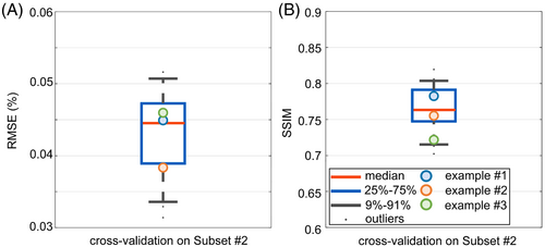
3.1 Model evaluation and selection
Table 1 contains the quantitative differences between the PR and the GT channel-wise -maps. Five neural networks were assessed for the corresponding subsets of the 5-fold cross-validation concerning the RMSE, SSIM, and symmetric loss. For example, the PR maps for unseen test subset 2 generated by network 2 yield a mean symmetric loss value of 0.0172, a mean RMSE value of 0.0438%, and a mean SSIM value of 0.7638 (Table 1). Similar results are observed for all five networks of the cross-validation. Network 2 yields the lowest mean value in the symmetric loss, the second lowest mean value in the RMSE, and the highest in the SSIM. Therefore, network 2 is selected for the performance analysis. The boxplot in Figure 3 depicts the performance of network 2 on all unseen slices from subset 2 regarding the RMSE (Figure 3A) and SSIM (Figure 3B). The performance of the network varies among slices ranging from 0.0314% to 0.0615% for the RMSE and from 0.7024 to 0.8195 for the SSIM. As representative examples, three of the 26 unseen test cases are visualized in the following with a high SSIM value of 0.7825 (example 1), a medium value of 0.7552 (example 2), and a low value of 0.7218 (example 3).
| NN | Training BMI mean ± SD (kg/m2) | Tested on | Test BMI mean ± SD (kg/m2) | RMSE mean ± SD (%) | SSIM mean ± SD | Symmetric loss mean ± SD |
|---|---|---|---|---|---|---|
| 1 | 23.57 ± 3.19 | Subset 1 | 23.99 ± 2.60 | 0.0440 ± 0.0064 | 0.729 ± 0.049 | 0.019 ± 0.003 |
| 2 | 24.06 ± 3.11 | Subset 2 | 22.12 ± 2.43 | 0.0438 ± 0.0067 | 0.764 ± 0.033 | 0.017 ± 0.002 |
| 3 | 23.42 ± 2.72 | Subset 3 | 24.53 ± 4.08 | 0.0435 ± 0.0096 | 0.727 ± 0.051 | 0.019 ± 0.004 |
| 4 | 23.48 ± 3.21 | Subset 4 | 24.37 ± 2.43 | 0.0449 ± 0.0063 | 0.734 ± 0.030 | 0.019 ± 0.002 |
| 5 | 23.76 ± 3.10 | Subset 5 | 23.15 ± 3.01 | 0.0518 ± 0.0084 | 0.728 ± 0.030 | 0.020 ± 0.004 |
- Abbreviations: BMI, body mass index; NN, neural network, RMSE, root-mean-square error; SD, standard deviation; SSIM, structural similarity index measure.
3.2 Evaluation of image quality
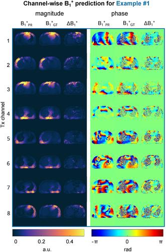
Figure 4 shows the channel-wise PR compared to the GT -maps for unseen example 1. The results for examples 2 and 3 are provided in the Supporting Information (Figure S1 and Figure S2). Qualitatively, the channel-wise PR matches the GT data not only for the magnitude, but especially for the phase distributions, which is a key requirement for subsequent pTx applications. A more detailed inspection of the magnitude difference (last columns in Figure 4) reveals larger differences in the chest region closer to the coil at Tx channels 1 and 8 compared to the other channels. This observation is consistent among subjects. A similar observation is not made with elements closer to the spine.
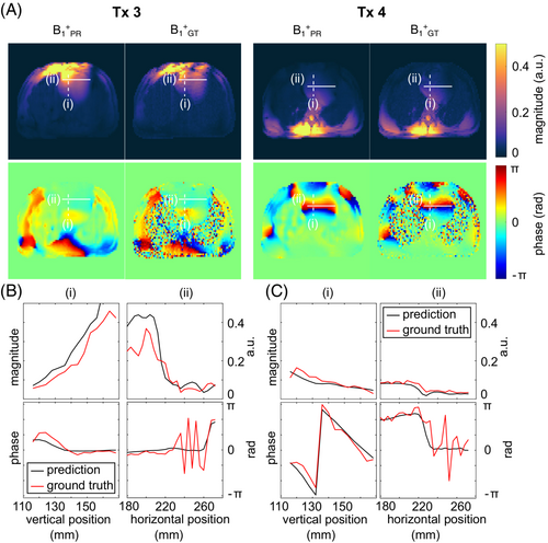
The observed match is further supported in Figure 5, showing a detailed view (Figure 5A) and a quantitative comparison (Figure 5B,C) between the PR and GT data for the third and fourth Tx channel for example 1. Line plots for cross-sections through the heart for magnitude and phase of the DL predicted (black) and measured (red) -maps are displayed. Although the magnitude and phase of the PR distributions follow the GT, sudden changes or edges (e.g., in the phase) are reflected less accurately by the prediction. This is not unexpected because neural networks minimizing distance metrics tend to smooth the data.45 The mean error for the magnitude (nRMSE, definition Plumley et al.29 ± SD) averaged over the cross-section amounts to 5.90% ± 8.87% for Tx channel 3 and 0.41% ± 1.01% for Tx channel 4, whereas the mean phase differences are 0.37 rad ± 0.38 rad for Tx channel 3 and 0.43 rad ± 0.50 rad for Tx channel 4.
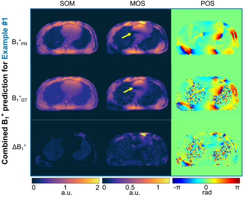
Similar results can be observed when the eight B1+-maps are combined for the three unseen test cases (Figures 6 and Supporting Information Figure S3). The network yields a prediction for example 1 with a mean error for the SOM over the heart of 0.69%, for the magnitude of the complex sum (MOS) of 3.86%, and with a mean difference in the phase of the complex sum (POS) of 0.015 rad. The pattern, i.e., the local signal dropouts and the corresponding phase wraps in the heart are approximated accordingly (see yellow arrows).
3.3 B1+-shimming performance
Figure 7 depicts the -shimming results for the three unseen test cases (examples 1–3) after calculating three -shim vectors based on the PR -maps that are applied to the PR and GT -maps. The results are shown for the default shim setting bDef (Figure 6), homogenous shim bHom, efficiency setting bEff, and the shim setting bEnf, when enforcing the mean efficiency to 50%.
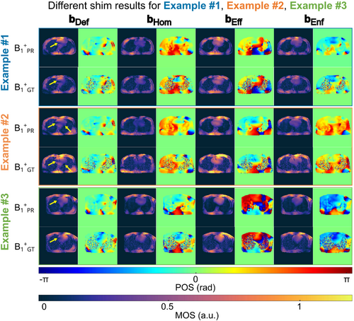
The default setting bDef (left column of Figure 7) calculated based on electromagnetic simulations yields different magnitude distributions among subjects, demonstrating the need for optimized pTx excitations. However, both PR and GT -maps show visually consistent results for all three subjects. Although bHom, tends to improve the homogeneity to the cost of lower magnitude values, the efficiency shim bEff leads to higher amplitudes but at the expense of stronger spatial -variation. In contrast, the enforced shim bEnf causes lower mean efficiency but also less pronounced dropouts, as seen in the bEff results. Importantly, all such features are always reflected by both the GT and PR maps. This high level of visual agreement among PR and GT maps is observed independently of the example and applied shim.
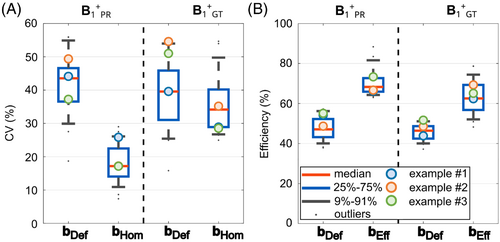
To investigate this agreement in more detail, a quantitative evaluation for the settings bHom and bEff are shown in Figure 8 for all 26 test cases of subset 2. When calculating a homogenous shim based on the PR maps (Figure 8A) the mean CV decreases from 43.5% (range = 18.7%–55.9%) to a value of 17.2% (range = 7.4%–29.0%). The mean decreases from 39.6% (range = 25.0%–54.6%) to 34.2% (range = 24.9%–54.6%) when applying bHom to the GT. Those CV values are overall higher for the GT compared to the PR case, but the CV values after shimming for both are lower than compared to bDef. For the efficient shim bEff, the mean efficiency increases from a mean value of 47.1% (range = 37.9%–57.2%) to a value of 68.3% (range = 63.0%–88.4%) for the PR maps. When applying the same vector to the GT, the mean efficiency increases from 46.4% (range = 37.2%–53.3%) to 62.5% (range = 48.3%–78.6%), leading to similar results for the GT and PR data.
3.4 Performance of the neural network in unseen test cases
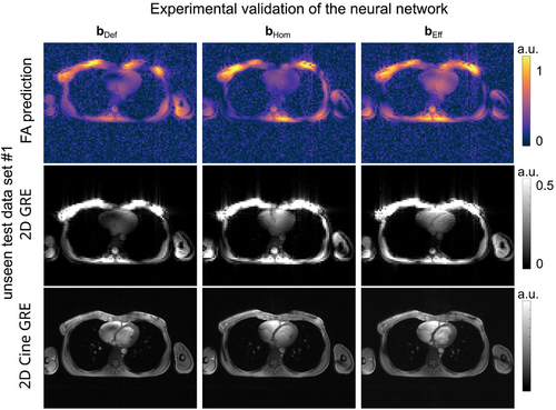
Figure 9 illustrates the FA prediction for the measured channel-combined -maps, the reconstructed 2D GRE image, and cardiac 2D cine GRE for the unseen test case 1 acquired with the corresponding pulses designed on the PR -maps. Qualitatively, a close match between FA predictions, the 2D GRE images, and cardiac cine images is observed, demonstrating the feasibility of the DL-based calibration approach. Similar results are obtained for two other subjects, illustrated in Supporting Information Figure S4. The results of the 5-fold cross-validation using all thorax geometries are provided in Supporting Information Table S1.
4 DISCUSSION
This work presents a novel, fast DL-based approach for obtaining relative -maps in the human heart at 7T, addressing the urgent need for reducing -calibration times in UHF body imaging. The data-driven approach predicts the 2D -maps in 0.2 seconds per slice from 2D localizer images typically acquired at the beginning of the session for planning. Therefore, this approach could make an additional -mapping scan obsolete. Although this proof-of-principle is applied to estimate only in a 2D slice, it may be extended toward multi-slice application and potentially to 3D. Thereby, it may save several minutes of calibration time and potentially several breath-holds.
Some related DL approaches in UHF imaging have been recently reported for subject-specific calibration of the transmit -fields.25-29 Abbasi-Rad et al.28 predicted channel-combined -magnitudes from a standard localizer to determine a FA scaling factor for adiabatic RF pulses. Plumley et al.29 used DL to predict the complex, channel-wise -maps of an 8 Tx channel head coil after motion based on an initially acquired set of -maps. Eberhardt et al.25 used a 2-to-16-fold under-sampled set of -maps for a 16 Tx channel head coil and used neural networks to augment a full set of 16 complex, channel-wise -maps. The presented work, in contrast, derives a complete set of complex, channel-wise -maps of an 8 Tx channel body coil from an initial localizer image and applies the technique to the human body at 7T.
The proposed network is based on a standard UNet architecture and translates complex, 32 Rx-channel-wise localizers () as input into complex, relative 8 Tx-channel-wise -maps. Early results of this study showed that the magnitude data could be retrieved with reasonable accuracy from the localizer. All features of the magnitude -maps were approximated accordingly. Only localized deviations were visible. The maps appear smoothed, likely introduced by the loss function during network training. The effect seems not to affect results or hinder shimming applications because the spatial variation of is smooth. Estimating the Tx phase turned out to be more difficult, which was also reported by Plumley et al.,29 and particularly the loss function and reference RF phase impacted the result. Although in a few cases very localized residual phase prediction errors are still observed at locations with rapidly changing phases or at singularities, an overall high similarity is observed between PR and GT phase patterns. This property is a prerequisite for any static and dynamic pTx applications.
The DL models were all trained on a considerably larger set of maps from 44 healthy subjects compared to previous work for the brain25, 28, 29 to account for stronger inter-subject variations of the thorax geometry.12 However, a shift in the training data regarding different property distributions (BMI, age, and gender) can lead to a bias in the performance of the network. For example, the performance was higher for subjects with smaller BMI due to a skewed distribution of BMIs in the training library toward lower values. Because the BMI distribution in Germany is shifted toward higher values (26.85 ± 4.95 kg/m2),46 simply increasing the data may further amplify the bias. A selection from a more representative sample of the general population is needed for the training data. Furthermore, maps from patients may need to be included to account for anomalies in the thorax geometry.
When evaluating the pulse design with a phase-only -shim setting optimized on the PR, all features in the magnitude and phase match when applying the shim vectors. For the homogeneity shim setting bHom, the CV on the GT is higher compared to the optimized PR for all test cases, which is likely because of the smoothing effect on the magnitude data for the PR. Nevertheless, the resulting CV values for the GT are lower for bHom than for the default setting bDef. For some test cases (Figure 7, example 1), optimizing the homogeneity still leads to localized signal dropouts in the heart. This observation, however, is consistent with our experience with previous studies that apply phase shimming to the human heart. The same observation is made in this work when relying on GT data used for calibration. If comparing the channel-combined PR and GT -maps after applying bEff or bHom, the match was higher for the efficient than for the homogeneous shim. The mean values for examples 1–3 regarding the SSIM, when applying bHom, were lower (0.7412) than compared to bEff (0.7569). Small phase deviations may explain this because an error in the phase is expected to impact a homogeneous shim more than an efficient shim.
Although this study successfully demonstrates the feasibility of deriving complex multi-Tx-channel -maps from localizer scans, the work is still subject to a few limitations. In this proof-of-concept study, only a single RF coil, a commercial body array coil with 32 elements (8 dipoles and 24 loop elements), has been used because this is the only available multi-Tx-channel coil at our center that can be applied in vivo. The same 32 elements are used for transmission and reception when operating this coil. In the Tx case, four elements (1 dipole and 3 loops) are combined with a fixed phase setting, whereas all elements acquire independently in the Rx case. This might be beneficial for this type of application because the 8 Tx -maps are derived from 32 Rx maps. Future investigations could also include other types of coils, for example, pure 8 Tx/8 Rx transceiver body coil arrays. Furthermore, the presented work investigates only 2D transversal slices, but oblique slices are typically required for practical cardiac applications. It is expected that changing the orientation will require new training data, and the performance of the method in oblique slices may be different. However, extending the method toward 3D coverage that allows FA optimization over a 3D volume can be considered. Covering multiple slices of 2D transversal B1+-maps is expected to be feasible, for example, by relying on serial data processing. The extension of this technique by estimating 3D -maps from 3D localizer data may be more challenging and requires further investigation.
As for other DL approaches, the performance of the present technique depends on the type of training data used. In the presented case, the GT -maps and, therefore, the PR were relative30 and biased by the square root of the proton density.19 Despite this limitation, such maps were chosen for this work because they have proven to perform well for various -shimming applications targeting the human heart or body.7, 31, 32 Future work may include the investigation of other -maps obtained by different mapping techniques.
Although further investigations are needed to investigate the full potential of this method, this proof-of-principle study demonstrates the feasibility of overcoming long calibration scans in a subject-specific calibration pipeline using DL. Together with other DL methods, this technique could serve as a plug-and-play like calibration solution for UHF imaging.
5 CONCLUSION
This study successfully demonstrates that DL approaches are highly suitable to predict 2D relative -maps from initial localizer scans in the human heart at 7T. The proposed approach reduces the calibration time for subject-specific pTx to less than a second. This work is expected to impact the progress of UHF body applications, which are hindered by stronger -variations compared to the brain and by longer calibration times. Based on this approach, a push-button in situ optimization embedded in the scanner's calibration routine may be feasible, potentially promoting the clinical applicability of body imaging at UHF in the future.
ACKNOWLEDGMENT
We gratefully acknowledge funding from the German Research Foundation SCHM 2677/2-1, SCHM 2677/4-1, and GRK2260-BIOQIC. Open Access funding enabled and organized by Projekt DEAL. Open Access funding enabled and organized by Projekt DEAL.
FUNDING INFORMATION
The German Research Foundation, Grant/Award Numbers: SCHM 2677/2-1, SCHM 2677/4-1 and GRK2260-BIOQIC.


