k-Space-based coil combination via geometric deep learning for reconstruction of non-Cartesian MRSI data
Abstract
Purpose
State-of-the-art whole-brain MRSI with spatial-spectral encoding and multichannel acquisition generates huge amounts of data, which must be efficiently processed to stay within reasonable reconstruction times. Although coil combination significantly reduces the amount of data, currently it is performed in image space at the end of the reconstruction. This prolongs reconstruction times and increases RAM requirements. We propose an alternative k-space-based coil combination that uses geometric deep learning to combine MRSI data already in native non-Cartesian k-space.
Methods
Twelve volunteers were scanned at a 3T MR scanner with a 20-channel head coil at 10 different positions with water-unsuppressed MRSI. At the eleventh position, water-suppressed MRSI data were acquired. Data of 7 volunteers were used to estimate sensitivity maps and form a base for simulating training data. A neural network was designed and trained to remove the effect of sensitivity profiles of the coil elements from the MRSI data. The water-suppressed MRSI data of the remaining volunteers were used to evaluate the performance of the new k-space-based coil combination relative to that of a conventional image-based alternative.
Results
For both approaches, the resulting metabolic ratio maps were similar. The SNR of the k-space-based approach was comparable to the conventional approach in low SNR regions, but underperformed for high SNR. The Cramér-Rao lower bounds show the same trend. The analysis of the FWHM showed no difference between the two methods.
Conclusion
k-Space-based coil combination of MRSI data is feasible and reduces the amount of raw data immediately after their sampling.
1 INTRODUCTION
Magnetic resonance spectroscopic imaging (MRSI) is an imaging modality with which to map various biochemical compounds noninvasively and in vivo. This method can, for example, reveal important information about the neurochemical underpinnings of brain diseases,1 which is unique compared with other imaging modalities.2 The recent development of spatial-spectral encoding and multichannel acquisition allow whole-brain (wb)MRSI scans in clinically attractive times at high field3, 4 and ultrahigh field.4, 5 However, the sheer size of the acquired raw wbMRSI data makes the full integration of the MRSI reconstruction on the image-reconstruction computers of current MR scanners challenging, both with respect to computing power and RAM requirements. State-of-the-art wbMRSI acquisitions generate raw data of up to about 100 GB per 15 minutes, the postprocessing of which must be fast enough to not interfere with subsequent MRI sequences.6 A particular problem is that the size of the raw data increases proportionally with the number of receive-coil elements, which has dramatically increased over the last two decades due to striking benefits of fast MRI techniques.7 The introduction of receive-coil arrays8 has not only improved the SNR of MRI considerably, but has enabled the development of parallel imaging technologies, which are currently an indispensable part of all clinical MRI protocols. All of these benefits rely on a proper characterization of the receive fields (ie, sensitivity maps) of the individual coil elements and consequential estimation of coil combination weights, which determine how to best combine the signals from different elements in the most SNR-efficient and artifact-free manner. For proton (1H) MRSI, the most successful coil combination approaches use not the actual water-suppressed data to derive coil combination weights, but rather, collect separate water-unsuppressed information,9-11 which provides much more accurate coil combination weights.
In recent years, deep-learning reconstruction of MRI has become a well-established field that uses a variety of techniques to perform reconstruction tasks.12 Conventional MRI turns the signal of high-abundant water and lipid protons into high-SNR images. Thus, MRI acquisition can be accelerated by violating the Nyquist criterion in regular (parallel imaging) or in irregular (compressed sensing) k-space undersampling patterns, which is a trade-off between speed and SNR efficiency. To restore the full k-space or to reconstruct an artifact-free image, analytical methods were originally proposed and have been established as indispensable tools for routine MRI.13-15 Thus, current efforts in deep learning–based MRI reconstruction focus on reconstructing undersampled MRI (primarily staying on the Cartesian grid). Zhu et al16 presented an approach in which k-space data acquired by any acquisition trajectory can be learned to be reconstructed into the image domain.
Within MRSI postprocessing pipelines, the coil combination step is the most critical reconstruction step with respect to reducing the amount of data. Currently, the coil combination for MRI (including MRSI) is performed in the image domain. This has a significant disadvantage. The data of each receive-coil element must be processed separately. In other words, for a 64-channel receive coil, for example, the same reconstruction steps have to be repeated 64 times; likewise, the RAM requirements are accordingly higher. The combination of all MRI data can be performed only after all the raw data have been sampled and reconstructed (including final 3D spatial Fourier transform).
The obvious solution to lowering the hardware demands is to perform the coil combination as early as possible in the postprocessing pipeline in native sensor space (ie, ungridded k-space). This would not only dramatically reduce the RAM requirements and make repetition of reconstruction steps obsolete, but allow performing the major workload “on the fly” (in parallel with data acquisition). However, especially for non-Cartesian k-space sampling, this poses a significant challenge with regard to finding the right k-space convolution kernel.17
In this study, we propose a k-space-based coil combination of non-Cartesian data through geometric deep learning. The output of the network is a multichannel non-Cartesian k-space, which after summation of all channels allows subsequent reconstruction through either conventional analytical methods or by other deep-learning methods, such as end-to-end reconstruction.16
2 THEORY
2.1 Coil combination
 (1)
(1) is the coil-combined signal at position
  ;
;  is a scaling constant at position
  ;
;  is the signal of the channel
  at position
  ;
;  is the noise correlation matrix between the channels
  and
and  ;
;  is the complex weight of channel
  at position
  . The scaling factor
  can be defined as follows:
 (2)
(2)The noise correlation matrix  is estimated from the sample noise matrix18 and can be directly applied to all the acquired data (prewhitening of data). From now on, it is assumed that all data are prewhitened.
 as the sensitivity map of channel m, the SNR of
  is maximized.8 For the MRSI data, the MUSICAL coil combination method9 has been shown to provide a useful approximation, in which coil combination weights are estimated from the first FID time point of water-unsuppressed MRSI data as follows:
 (3)
(3) (4)
(4) (5)
(5) is the acquired signal in k-space domain and the second term inside the sum is the k-space of the approximation of the sensitivity maps. The second term can be replaced by the ESPIRiT version19 to suppress anatomical contrast and thus provide a better estimate for the sensitivity maps.
Equation 5 shows that the convolution is a natural operator for coil combination in k-space domain. A full convolution would be time-intensive, but because sensitivity maps are inherently smooth in spatial variation (ie, most of the information is concentrated in the k-space center), a truncated kernel can be used analogously to k-space-based parallel imaging reconstruction (eg, GRAPPA). The aforementioned convolution of multichannel data with a kernel is, in principle, possible, but it would be very challenging to handcraft the optimal kernel and it would require prior gridding on a Cartesian k-space grid, if non-Cartesian sampling trajectories (eg, spirals or concentric ring trajectories) have been used. Geometric deep learning can overcome both these challenges by (1) handcrafting the optimal kernel and (2) doing so for any arbitrary k-space geometry.
2.2 Geometric deep learning
Geometric deep learning20 is a general extension of deep-learning methods for data represented as graphs or manifolds. Convolutional neural networks rely on convolution operators, which allow the extraction of relevant features from input data.21
 (6)
(6) defines the number of nodes in the graph;
  defines the edges between the nodes of the graph; and
  is the adjacency matrix for which
  ,
,  .
. and convolution parameter
  can be defined as
 (7)
(7) acting over the graph function (features)
  is defined as
 (8)
(8) are pseudo coordinates of the nodes
  in the neighborhood of node
  , while the weighting function of the path operator is defined as
 (9)
(9) is a mean vector of the Gaussian kernel and
  is its covariance matrix. Both are learnable parameters.
In the context of the coil combination of non-Cartesian MRSI data (represented as a graph [Equation 6] with acquired signals of particular coil elements represented as  ), the convolution operator
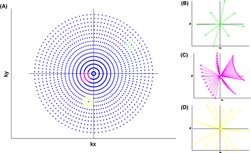
  of Equation 7, as presented previously, acts over the non-Cartesian data and provides a solution for how to approximate the coil combination in k-space without the need to grid data to a Cartesian grid (Equation 5). Figure 1 illustrates how kernels are defined for concentric ring trajectories in a 2D non-Cartesian k-space, including all connected nodes.
3 METHODS
3.1 Experimental data
All measurements were carried out on a 3T Prisma MR scanner with a 20-channel receive head/neck coil array (Siemens Healthineers; Erlangen, Germany). Twelve volunteers (7 males and 5 females) were included in this study. Internal review board approval and written, informed consent were obtained for all volunteers.
For each volunteer, rapid non-water-suppressed MRSI was performed, with the head of the volunteers placed in 10 different positions inside the coil. This is necessary to ensure that the trained neuronal network generalizes well for all possible heads and head positions with respect to the coil. The volunteers were measured with the following short-TR FID-MRSI sequence parameters23, 24: FOV = 220 × 220 × 200 mm³; volume of interest = 220 × 220 × 100 mm³; TR = 60 ms; acquisition delay = 1.3 ms; nominal flip angle = 16º; vector size = 16 complex points; spectral width = 1030 Hz; and acquisition time = 20 seconds. In-plane (kx, ky) encoding was performed by 16 concentric ring readouts using sine-modulated and cosine-modulated gradients. Through-plane (kz) encoding was achieved through 25 phase encodings. The target reconstruction matrix was 32 × 32 × 25, with a resolution of 6.9 × 6.9 × 8.0 mm³ without violating the Nyquist criteria.
An additional water-suppressed, long-TR FID-MRSI sequence was measured at the eleventh position with slightly modified parameters: TR = 470 ms; nominal flip angle = 50°; vector size = 360 points; and acquisition time = 3:11 minutes. All other scan parameters were identical.
Additional MPRAGE25 sequences with a nominal resolution of 1.1 × 1.1 × 1.0 mm³ were scanned within 2:38 minutes each, at two positions, for anatomical reference (ie, the first identical to the position of the first MRSI scans and the second identical to the eleventh MRSI scan).
3.2 Training and testing data preparation
Training data were derived only from the short-TR MRSI data without water suppression.
The fast Fourier transform in the partition direction was performed and the volume of interest was masked. Then, the data were transformed back to full k-space. These steps were consistently applied to all in vivo MRSI data.
 (10)
(10) is the number of time points,
  , and dwt is the dwell time. The phase offset maps should eliminate dependency of the sensitivity maps’ phase information on the B0 inhomogeneity, which helps following the ESPIRiT algorithm to estimate sensitivity maps.
 (11)
(11) is the magnitude of the first FID point.
The estimated sensitivity maps were applied to reconstructed, non-water-suppressed MRSI data, which had been augmented with the two following steps: (1) A random phase was added, sampled from the uniform distribution, <-π, π>; and (2) the magnitude of the MRSI data was randomly scaled, sampled from the uniform distribution, <0, 1>. Those two steps were repeated twice for each data set. All data were then transformed back to non-Cartesian (kx, ky) k-space coordinates through the discrete Fourier transform. Then, the FFT was applied in the (kz) partition direction. In addition, a Hamming filter and an annihilation filter26 were applied in the kx and ky dimensions.
Using this procedure, pairs of non-Cartesian k-space training data were generated. Each instance consisted of only one partition encoding step and one FID point. Each pair consisted of (1) the input to the network, which was corrected by the FOV shift and the phase-roll shift, and (2) the desired output of the network, which was also corrected by the sensitivity maps. Thus, the desired output was defined as the k-space representation of the data right before the summation step of the coil combination.
Training data were obtained only from 7 of 10 volunteers. The data of the remaining 3 volunteers were used for further analysis of the network performance.
For testing, the long-TR MRSI data (with activated water suppression) of the eleventh head position were used. The preprocessing consisted only of the FOV shift, the off-resonance correction, and the spatial filters (same as for training data).
3.3 Neural network architecture
The non-Cartesian data were represented as a graph. The nodes of the graph represent acquired points in k-space with unique coordinates. These k-space coordinates were normalized, and the Euclidean distances between all nodes were calculated. An edge between two nodes was created if the distance between those nodes was lower than 1.5 times the Nyquist criterion. The graph connectivity is depicted in Figure 1. The edge was weighted by the inverse of the Euclidian distance between two nodes. The complex values of acquired signals were separated into real and imaginary parts and are represented as separate features of the nodes. Therefore, the number of features per node was twice the number of coil elements.
A shallow-graph neural network was designed in Deep Graph Library consisting only of two Gaussian mixture model convolution layers,22 which are described in section 2. Gaussian mixture model convolution layers with 10 Gaussian kernels were chosen. Bias terms were not used for either layer, and a tanh activation was used after the first layer. The pseudo-coordinates of nodes in the neighborhood were defined in Euclidean coordinates. The number of input and output features for the whole network was equal, while the output of the first convolutional layer had only half of the input features. The input and desired output were also weighted by an annihilation filter.26
3.4 Network training
The training and the following inference of the network with the data was performed using a Tesla V100 GPU (Nvidia; Santa Clara, CA). The Deep Graph library27 was used with the PyTorch28 DL framework.
Training of the neural network was separated into two parts. First, the network was trained to perform the coil combination task without introducing any noise. Then, the network was fine-tuned by adding white noise to the input data to make the performance of the network more robust against noise.
The first training consisted of 50 epochs with batch size = 10. The Adam optimizer was used with a learning rate of 1−4. The loss function was the mean squared error.
The second training consisted of 30 epochs. The Adam optimizer was used with a learning rate of 1−4. The same loss function and batch size as in the first training were used. White Gaussian noise was simulated for each instance and epoch with a zero mean. The SD of the noise was randomly sampled from the uniform distribution <0.1> scaled by 0.0001 of the absolute maximum in the data set and by the number of the current epoch. The spatial filters (the Hamming and annihilation filter) were applied after the addition of noise.
3.5 Evaluation
To evaluate the performance of the network, water-suppressed long-TR MRSI data were used. The analysis was carried out on 4 volunteers: (1) the first volunteer whose water-unsuppressed MRSI data were included in the training data set, but not the water-suppressed MRSI; (2) the second volunteer for whom no data were ever shown to the network; (3) the third volunteer was measured with seven head positions following a “head shaking” motion and five head positions following a “nodding” motion; (4) the fourth volunteer was measured at the same position with nine averages. From these nine averages, three data sets were generated and evaluated to simulate different SNR regimes: one average (standard SNR), four averages (double SNR), and all nine averages (triple SNR). Again, data of the third and the fourth volunteer were never used during the training of the network.
Directly after prediction, the annihilation filter was removed from the output data. The data were then summed across the channels and Hamming-filtered in the partition direction. The resulting single-channel data were then reconstructed into the image space using our standard reconstruction,24 and spectra were fitted using established MRS quantification software (LCModel29), with the basis set including 16 metabolites and a macromolecule baseline adapted for 3 T.30
From the output of the LCModel, the ratio maps were calculated and the Cramér-Rao lower bounds of three main metabolite groups (tCr [total creatine], tNAA [N-acetylaspartate + N-acetylaspartyl glutamate], and tCho [total choline]) were directly obtained. The SNR of the NAA and tCr resonances were estimated from the respective LCModel fits. For this, the maximum of each metabolite fit was divided by the SD of the noise from a metabolite-free spectral range (ie, approximately 7.68-6.52 ppm). Smooth baseline variations in this spectral range were estimated by a polynomial fit of the fourth order and subtracted. The residuum was analyzed for normality by a Kolmogorov-Smirnov test ( ) to identify possible remaining artifacts. The FWHM of tCr was calculated from the LCModel fit.
The results of the k-space coil combination (kspCC) were compared with a conventional image-based coil combination (cCC) termed “iMUSICAL.”9, 11
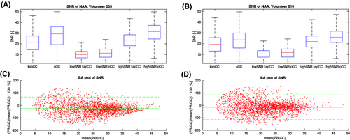
The SNR results of the methods were compared by Bland-Altman plots,31 but with replacement of the more common absolute difference of the two compared values by their relative difference (in percentage). The mean of the two methods was taken as the denominator.32 The absolute values of the SNR of NAA were compared by boxplot analysis. The SNR evaluation was performed separately for low-SNR (< 15) and high-SNR (≥ 15) data, as Bland-Altman plots indicated a systematic SNR-dependent performance difference.
The results of the FWHM of tCr were compared by Bland-Altman plots in the same way as for the SNR analysis. The boxplots were computed for a quantitative analysis over the whole volume. The CRLBs of the three main metabolites (tNAA, tCr, and tCho) were compared between both methods using boxplots. The relative metabolite maps of tNAA/tCr and tCho/tCr were qualitatively compared between two methods only for the volunteer whose data were not used during the training process. Sample spectra of the same volunteer were qualitatively compared between both methods.
4 RESULTS
4.1 Spectral data quality
The spatial distributions of the SNR values of two metabolites (NAA, Cr) were very similar for both methods in all three orthogonal projections (Figure 2). Quantitative results for the SNR (NAA) of the 2 volunteers indicated that cCC outperformed the kspCC overall, but this SNR difference between both methods was driven by the high SNR regions (Figure 3A,B). The Bland-Altman plots show that the difference in the SNR values of both methods is not homogeneous across the whole range of SNR values (Figure 3C,D). Although there was an overall higher SNR for cCC (median = 29, interquartile range [IQR] = 20-36) over the whole volume of volunteer 5 than for kspCC (median = 22, IQR = 15-28), no difference was found for the low-SNR regime (cCC: median = 9, IQR = 7-12; kspCC: median = 10, IQR = 7-14). The same pattern was observed for volunteer 10. Again, the overall SNR was higher for cCC (median = 24, IQR = 16-29) than for kspCC (median = 19, IQR = 13-27), but there was no difference in the low-SNR regime (cCC: median = 12, IQR = 10-14; kspCC: median = 12, IQR = 9-14). The Bland-Altman plots showed a systematic offset for both volunteers (volunteer 5: mean = −20% with 1.96*SD of 90%; volunteer 10: mean = −15% with 1.96*SD of 90%) in favor of the cCC, which was driven by a larger population of high (> 20) SNR values. A correlation analysis showed that this SNR difference increased linearly for higher SNR values.

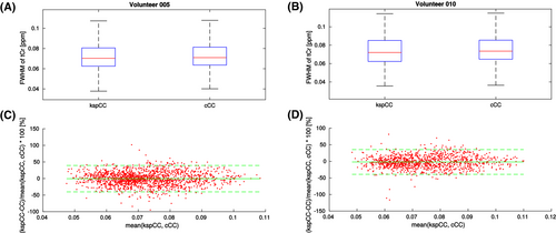
The FWHM maps of the tCr depicted in all three orthogonal projections at the same location as for the SNR maps showed a similar spatial distribution of FWHM values (Figure 2). The boxplots for the FWHM values over the whole volume (Figure 4A,B) showed no difference between both methods for either volunteer 5 (cCC: median = 0.071 ppm, IQR = 0.063-0.081 ppm; kspCC: median = 0.070 ppm, IQR = 0.062-0.080 ppm) or volunteer 10 (cCC: median = 0.073 ppm, IQR = 0.064-0.085; kspCC: median = 0.072 ppm, IQR = 0.062-0.085 ppm). The Bland-Altman plot (Figure 4C,D) showed negligible offsets between methods (volunteer 5: mean = −0.4% with 1.96*SD of 39.8%; volunteer 10: mean = −1.9% with 1.96*SD of 37.3%).
4.2 Spectral fitting quality
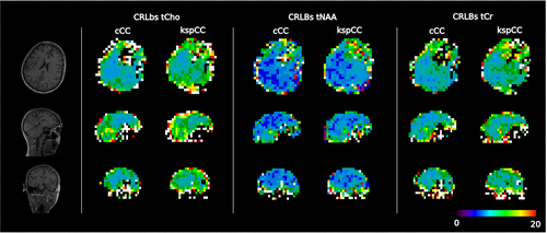
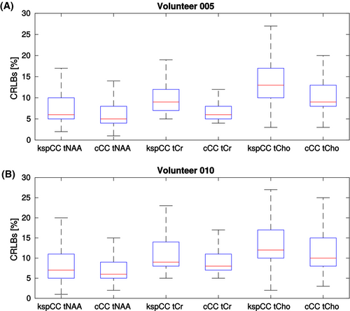
Qualitatively, the spatial distributions of the CRLB values of the three metabolites (ie, tCho, tNAA, and tCr) for both methods were similar (Figure 5); however, consistent with the observed SNR differences, the CRLBs of all three metabolites groups were lower for cCC than for kspCC (Figure 6): The median CRLB of tNAA of volunteer 5 for kspCC was 6% with an IQR of 5%-10%, whereas, for cCC, the median was 5% with an IQR of 4%-8%. The same pattern was observed in results of volunteer 10: For kspCC, the median CRLB of tNAA was 7% with an IQR of 5%-11%, and for cCC, the median CRLB of tNAA was 6% with an IQR of 5%-9 %. The median CRLB of tCho for volunteer 5 for kspCC was 13% with an IQR of 10%-17%, and for cCC, it was 9% with an IQR of 8%-13%. Again, the same pattern was observed for volunteer 10: For kspCC, the median CRLB of tCho was 12% with an IQR of 10%-17%, and for cCC, the median CRLBs of tCho were 10% with an IQR of 8%-15%.
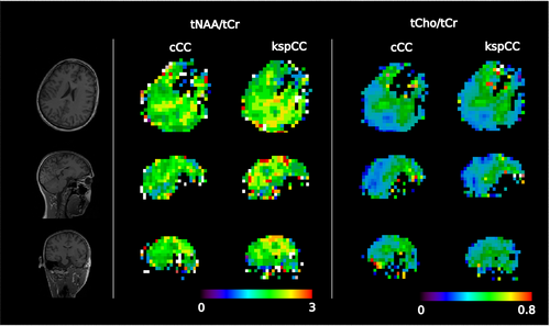
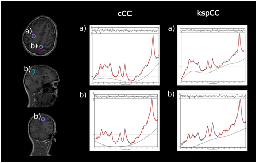
Qualitatively, the contrast of the metabolic ratio maps from both methods, kspCC and cCC, were similar in all three orthogonal projections (Figure 7). Sample spectra of both methods were similar except for differences in the baseline (eg, volunteer 10) (Figure 8).
4.3 Stability of the network performance against extreme head positions
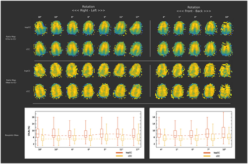
The performance of the network was robust against position changes (ie, head rotations) over the entire range possible within the limitations imposed by the coil dimensions. This included “head shaking” motion over a range of −17 to +18° relative to a neutral initial position (Figure 9; left column). Metabolic ratio maps were similar for both methods. The CRLBs of tNAA for cCC were same for all positions. For kspCC, the CRLBs of tNAA increase by +1%. The performance of both methods for positions followed the “nodding” motion pattern were also stable over a range of −4 to +10° (the CRLBs of tNAA for cCC remained unchanged; the CRLBs for kspCC increased by 1%) with no major change of metabolic ratio maps (Figure 9, right column). However, B0-shimming errors due to strong motion resulted in consistently worse data quality in the frontal lobe for both approaches.
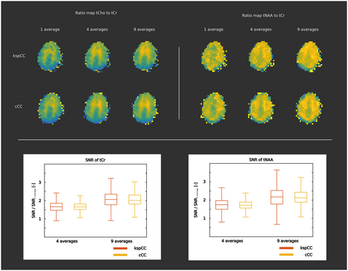
4.4 Performance of the network in various SNR regimes
The quality of metabolic ratio maps increased linearly with the number of averages for both methods (Figure 10, top section). For both methods (Figure 10, bottom section), the increase of the SNR of tCr between one average and four averages was similar (for cCC: median = 1.66, IQR = 1.51-1.81; for kspCC: median = 1.66, IQR = 1.46-1.85). The SNR of tNAA between one average and four averages followed the same pattern (for cCC: median = 1.72, IQR = 1.56-1.89; for kspCC: median = 1.75, IQR = 1.50-1.97). The increase in the SNR of tCr (for cCC: median = 2.01, IQR = 1.81-2.30; for kspCC: median = 2.05, IQR = 1.77-2.35) and the SNR of tNAA (for cCC: median = 2.12, IQR = 1.89-2.43; for kspCC: median = 2.17, IQR = 1.78-2.53) between one average and nine averages was also similar for both methods.
5 DISCUSSION
This paper presents the first proof-of-principle of a k-space-based coil combination method. The major benefit of this method is that the signals from all coil elements can be combined in any native sensor space (eg, non-Cartesian k-space) without the need to perform a Fourier transformation to the image space beforehand. This shifts the major reconstruction workload to the sequence run-time and eliminates the need for excessive RAM requirements. Ultimately, this makes fully reconstructed MRSI or MRI data available immediately after the acquisition is finished.
Lately, many deep learning–based reconstruction methods were proposed for MRI,12 focused primarily on reconstruction of undersampled Cartesian k-space MRI data by restoring the missing k-space points or by correcting the image artifacts, which are caused by the violation of the Nyquist criterion.
The acceleration of MRSI acquisition through undersampling of the k-space is possible,33 but the acceleration through spatial-spectral encoding34-37 is more efficient in terms of speed and can yield higher SNR, thus enabling high-resolution wbMRSI in reasonable time frames. Spatial-spectral encoding can still be combined with parallel imaging, making the reconstruction even more complex, but is recommended rather as an add-on.11, 38 A disadvantage of spatial-spectral encoding is the amount of generated raw data, especially if non-Cartesian spatial-spectral encoding techniques are used. For high-spatial and spectral-resolution MRSI, these can be more SNR-efficient and time-efficient than their Cartesian counterparts, but have the disadvantage of an even more complex reconstruction. Furthermore, the amount of raw data is linearly proportional to the number of receive coil channels. Currently, the use of 64-channel coil arrays and beyond is becoming a new standard in the detection of human brain pathology.7
Conventional neural networks assume a regular/equidistant/grid-like structure of the data or such representation (eg, non-Cartesian acquisition trajectories can be represented as a vector16). Our coil combination approach uses geometric deep-learning methods. Geometric deep learning offers the generalization of deep-learning methods over the data represented as a graph, where also structure of the data is an input variable. Such methods allow input of data with various structures (in principle, one network could potentially process MRSI data acquired with different non-Cartesian trajectories).
In our case, the coil combination task is performed over non-Cartesian data. The MRSI data were neither gridded on the Cartesian grid nor transformed to any other domain. The k-space coil combination network was able to combine the MRSI data of volunteers, one of whose data were never shown during the training. This is in contrast to currently used coil combination methods in the MRSI field, which are performed exclusively in the image domain and rely on estimation of sensitivity maps or similar external or internal prescans9, 39, 40 or are data-driven, such as whitened singular value decomposition.41 Such generalization was achieved by the acquisition of water-unsuppressed data at the different head positions of different volunteers inside of the coil, which formed the basis for simulation of training data. To the best of our knowledge, this is the first published coil-combination method in the k-space domain for MRI or MRSI.
The inference of the network per partition (all FID points) took about 2 seconds. Each partition consisted of 16 concentric rings, thus resulting in an inference of about 125 ms per TR, which is approximately one-fourth that of the TR used for acquisition (TR = 470 ms). Although this is sufficiently fast for possible online reconstruction, further optimization will be important to allow rapid online signal combination for even shorter TRs.5, 42
The results of the SNR analysis suggest that the SNR over the whole brain is overall lower when using kspCC compared with the cCC. The spatial distribution of SNR values was very similar for both methods, as well as for a metabolite close to the problematic lipid region in proton spectra (eg, NAA) and for a metabolite more distant from the lipid region (eg, tCr). Thus, extracranial lipid artifacts can be ruled out as a source of error in the SNR assessment.43 A more detailed analysis revealed that there is no noticeable SNR difference for low SNR values, but there is a pronounced difference between kspCC and cCC in the high SNR regions. However, the analysis of data with a different number of averages revealed a similar increase of SNR for both methods with increasing number of averages. Those two results suggest a more complex causality between the level of noise and performance of the network. Fortunately, typical wbMRSI sequences are optimized for high spatial resolution with just acceptable enough SNR to guarantee adequate spectral quantification. As long as the SNR is good enough in the worst brain regions, an SNR loss in the best regions is acceptable. This lower SNR difference in the low-SNR regions could have been the result of the two-step training of the neural network. This pattern was consistent for volunteers, regardless of whether the network had ever seen any kind of data from the particular volunteer. Further investigation of this unexpected effect will be necessary.
The results of the FWHM analysis showed that there was no difference between either coil combination method with respect to spectral linewidth. The spatial distribution on the FWHM maps, the boxplots, as well as the Bland-Altman plots, suggested a very similar performance.
The CRLB values are known to be affected by spectral SNR.44 Thus, the results of the CRLBs of the main metabolite groups (tNAA, tCr, tCho) showed a similar discrepancy for low CRLB values for kspCC. This trend could be observed in the CRLBs map and was directly visible through the boxplot analysis. The CRLB of each metabolite represented the quality of fit (ie, precision) and depended not only on the SNR, but also on the spectral overlap of neighboring resonances and the presence of spectral artifacts. A common practice in automatic quality assurance is to threshold the volume with a reasonable CRLB (eg, metabolite quantification with CRLBs ≤ 20% or, in some cases, ≤40%, are considered acceptable). Thus, an increase in very low CRLB values does not constitute a major problem for further analysis.
The final results of MRSI quantification included metabolite ratio maps. Our results showed that the spatial distribution of tNAA/tCr and tCho/tCr were very similar in all orthogonal slices for both coil combination methods. These results suggest a similar performance and the same information content, no matter which coil combination method was used.
This work describes the first proof-of-principle of the coil combination method in the k-space domain. Conventional kernel-based k-space-based coil combination, similar to the gridding algorithm, may introduce artifacts in the image domain, as described by Lustig et al.45 However, the task performed by a neural network is defined by a training data set, which could include ways to to correct for coil sensitivities profiles as well as any other required correction terms. Thorough investigation of such effects is further required.
Further optimization of the network architecture and generalization to different coils and MR scanners will be necessary. Currently, our neural network is limited to only one spatial resolution and a fixed FOV. Therefore, only a network architecture that consisted of two convolutional layers was necessary. We expect that, with increasing variety of input data (such as different FOV or spatial resolution), the complexity of the network would need to be increased (such as by adding more layers). The network was designed for a particular coil with a fixed number of channels and geometry. The number of channels defines the number of features per node. However, all channels are not always active during acquisition. The performance of the network in such cases needs to be further investigated. The graph representation of the MRSI data was very simple and driven by the MRSI physics (ie, definition of node neighborhood according to the Nyquist criteria).
Further optimization in the graph representation is possible. The time dimension of the MRSI data along the FID evolution was not taken into account. Currently, each single FID time point is processed independently, but the character of MRSI data suggests that the information of one time point is related to the information present in earlier, as well as later, time points. This information could be exploited to further improve reconstruction (eg, SNR) in the future.
A fairly small number of volunteers (n = 12) was recruited. Moreover, sensitivity profiles required to coil-combine the MRSI data were learned from only 10 different head positions per volunteer inside the coil. The remaining data were created through data augmentation. More training data with a higher variability may improve these results.
After further improvement of the k-space coil combination, the reproducibility study and thorough comparison against a higher number of available coil combination methods needs to be performed. Such studies would clarify the benefit of the proposed method against the conventional method.9, 41, 46
The CRLB is specific to the unbiased estimator,47 which cannot be said about the deep-learning methods. Further evaluation of the precision and the accuracy of the method needs to be performed in which the ground truth is known.
6 CONCLUSIONS
This paper presents the preliminary results of a new coil combination approach for MRSI data, which is performed in native non-Cartesian space before gridding on Cartesian coordinates. Geometric deep learning was used to solve this reconstruction step. Considering the preliminary nature of our study, the results are highly promising and open the possibilities to move many postprocessing steps into the raw sensor space (eg, undersampled k-space reconstruction), which would ultimately lead to rapid online reconstruction for clinically attractive wbMRSI.
Open Research
DATA AVAILABILITY STATEMENT
The main part of the code will be available on Github (https://github.com/stanomot/kSpace-coil-combination-of-nonCartesian-MRSI-data). For more detailed questions, the readers are encouraged to contact the authors.


