Copolymerization of VDF and HFP in Supercritical Carbon Dioxide: A Robust Approach for Modeling Precipitation and Dispersion Kinetics
Abstract
A kinetic model is developed for the heterogeneous free-radical copolymerization of vinylidene fluoride and hexafluoropropylene in supercritical CO2. The model accounts for polymerization in both the dispersed (polymer-rich) phase and in the continuous (polymer-free) supercritical phase, for radical interphase transport, diffusion limitations, and chain-length-dependent termination in the polymer-rich phase. A parameter evaluation strategy is developed and detailed to estimate most of the kinetic parameters a priori while minimizing their evaluation by direct fitting. The resulting model predictions compare favorably with the experimental results of conversion and MWD at varying monomer feed composition, monomer concentration, interphase area, and pressure of the system.
1. Introduction
Since the work of DeSimone et al.,1 supercritical carbon dioxide (scCO2) attracted a lot of attention as green polymerization medium alternative to water and volatile organic solvents. It is in fact cheap and abundant, nontoxic, nonflammable, and does not undergo chain transfer reactions. A major drawback of the process is the need of high pressure (typically few hundred bars). Nevertheless, such drawback is somehow counterbalanced by the easy recovery of very pure polymer by simple depressurization at the end of the reaction, without any need of polymer purification steps. Many papers and reviews have been published addressing the main features of the polymer/scCO2 thermodynamics,2, 3 as well as those of polymer synthesis, modeling of polymerization kinetics, and polymer processing in scCO2.4-11
Because of the poor solubility of many polymers in scCO2, radical polymerizations in such medium are almost always carried out under heterogeneous conditions (below the polymer cloud point pressure and temperature). Low-molecular-weight monomers and initiators are soluble in scCO2 and the reaction starts under homogeneous conditions. As the reaction proceeds, the polymer phase separates and the reaction proceeds in the presence of two phases: the continuous CO2-rich phase and the dispersed polymer-rich phase,12, 13 with monomers (and initiator) partitioned between the two.
In recent years, the heterogeneous free-radical homopolymerization of vinylidene fluoride (VDF) and its copolymerization with hexafluoropropylene (HFP) have been the subject of several experimental studies. Precipitation,14-17 as well as dispersion polymerizations18-22 have been analyzed. The reason of such an interest is twofold. First, VDF–HFP semicrystalline copolymers are technologically relevant materials, mainly because of their chemical and thermal stability.23-25 Second, precipitation reactions carried out in scCO2 show a very distinctive feature: when monomer concentration exceeds a threshold value of about 2 mol · L−1, the copolymer produced is characterized by a bimodal molecular weight distribution (MWD).15-18
Recently, Costa et al.18 compared the MWDs of copolymers produced under precipitation (smaller value of the interphase area) and dispersion (larger value of the interphase area) conditions. They found that the amount of interphase area, Ap, between the precipitated polymer and the continuous CO2-rich phase, affects the bimodal MWD of the produced copolymer: the larger the value of Ap, the larger the relative amount of the higher-MW mode. This finding proves that the interphase area has a profound effect on the reaction kinetics and qualitatively supports a previously proposed 2-loci kinetic model, successfully applied to the VDF as well as to the methyl methacrylate (MMA) homopolymerizations in scCO2.16, 26, 27 In the frame of such model, the two modes in the MWDs are representative of the polymer produced in each one of the two phases, i.e., the CO2-rich phase and the polymer-rich phase.
Accordingly, in this paper the 2-loci model is extended to the copolymerization of VDF and HFP in scCO2. A parameter evaluation approach different from that used by Mueller et al.16 is also proposed to simplify the use of the model. The paper is organized as follows: model assumptions and equations are presented in Section 2. The procedure of parameter evaluation is discussed in Section 3: it is shown that despite the very large number of model parameters most of them could be determined from independent experimental measurements or physically sound arguments. As a result, the number of adjustable parameters was minimum and their value tuned using a limited number of experimental MWDs. In Section 4, model predictions are compared to experimental results: the effects of feed composition, interphase area, reaction time, and pressure on the complete MWD are considered, showing remarkable model prediction power in all cases. In Section 5 it is shown that the heterogeneous model describes well also the MWDs obtained under precipitation conditions in a continuous stirred-tank reactor (CSTR).
2. Model Development
We kept essentially unchanged the main assumptions underlying the kinetic model previously developed for the precipitation reaction of VDF in scCO2.16 Accordingly, only the most important model assumptions, together with the resulting equations, are reported in the following.
2.1. Phase Behavior
- (i)
The reaction volume VR is considered to be composed of three phases. One is the CO2-rich continuous phase (sc phase) of volume Vsc. The other two are the amorphous (pa phase), of volume Vpa, and the crystalline polymer phase (pc phase), of volume Vpc. The total polymer volume is represented as composed of Np particles with the same average volume vp:
 ((1))
((1))Also the crystallinity degree, Xcr (defined on a mass basis), is the same for all particles. From here on, we indicate with the superscript i = (sc, pa, pc) the corresponding phase; the whole copolymer, made of crystalline and amorphous portions, is denoted by the superscript pol.
- (ii)
Low-molecular-weight components (monomers, carbon dioxide, and initiator) are in thermodynamic equilibrium between the sc phase and the pa phase, while the crystalline polymer is considered completely impermeable to all species. Therefore, both Vsc and Vpa contain initiator and monomers and are possible reaction loci.
- (iii)
Due to monomers and initiator partitioning, growing radical chains are generated in both phases and, depending on their partition and transport coefficients, undergo mass transport across the interphase area. Accordingly, radicals growing in one phase, may propagate up to termination in the same phase, or diffuse into the other phase where they may go on growing and eventually terminate.
- (iv)
Poly(vinylidene fluoride) (PVDF)-based polymers have extremely low solubility in the CO2-rich phase at experimental conditions close to those considered in this work (T = 50 °C, P < 400 bar, fHFP < 0.3).15, 28, 29 This consideration applies also to low-MW chains.30, 31 Therefore, polymer formed in the continuous phase eventually accumulate in the dispersed one (assumption of zero solubility of dead chains in the sc phase).
- (v)
For VDF–HFP precipitation reactions, Beginn et al.15 observed an onset in turbidity in the polymerization medium due to polymer precipitation already after the first few minutes of reaction. Since at that stage the conversion is still very low, such observation implies a fast nucleation stage. Accordingly, we consider the nucleation stage to occur instantaneously at very low conversion (Xnucl = 0.001), thus forming a given number of particles, Np, which remains constant all along the reaction. At conversion smaller than Xnucl, the reaction system is considered homogeneous.
2.2. Reactions
- (vi)
The “long-chain approximation” (LCA) is applied. This allows one to estimate the fraction of radicals whose reactive unit is a VDF or an HFP group. This way the population balance equations (PBEs) can be written in terms of composition averaged rate constants, as detailed in Appendix A.
- (vii)
No chain transfer to polymer takes place in the continuous sc phase, and a chain-length-independent termination rate constant is assumed in the same phase. On the contrary, both chain transfer to polymer as well as a chain length dependent termination rate constant are operative in the dispersed pa phase. This is a direct consequence of assumption (iv): since the polymer precipitates out of the sc phase, transfer to polymer cannot occur in that phase, the viscosity of the medium remains low and the termination rate constant can be considered length-independent. On the contrary, the high polymer content in the pa-phase enhances the role of chain transfer to polymer reactions,32 as well the effect of diffusion limitations on the reaction rate constants.
- (viii)
For both phases, termination by combination only is considered because there is no evidence in the literature on disproportionation.17 The values of all homo- and cross-termination rate constants have been assumed equal.
2.3. Comments
The different behavior in terms of partitioning between radicals and other species (low-MW components and polymer chains) is due to the different ratio between the characteristic times of termination and diffusion. Depending on the reaction conditions, the timescale of radical termination may be comparable to that of interphase transport making the two processes competitive so that no equilibrium partitioning can be achieved.16, 26 On the other hand, the lifetime of VDF, HFP, initiator (I), CO2 and dead chains, is comparable to the reaction duration and equilibrium conditions are easily established.
When bimodal MWDs were obtained for poly(VDF-co-HFP) synthesized in scCO2, the low-MW peak, attributed to polymer formed in the continuous phase, is typically narrower than the high-MW peak.16-18 This evidence supports the assumption that chain transfer to polymer and diffusion limitations for the termination events are negligible in the continuous phase (assumption vii) since both events lead to broadening of the MWD.
2.4. Thermodynamic Modeling
No data about initiator partitioning are available. Therefore, equipartitioning of diethylperoxidicarbonate (DEPDC) was assumed at all operative conditions, i.e.,  equal to one,
  being the weight fraction of the initiator in phase i. The partitioning of monomers and CO2 between Vsc and Vpa was modeled by the Sanchez-Lacombe (SL) molecular theory.33-35 In the following, the subscript c indicates a generic component (VDF, HFP, CO2, or the amorphous copolymer fraction).
 ((2))
((2)) ((3))
((3))Accordingly, only three parameters out of the six mentioned are truly independent. In Equation 2 and 3, ρ* is the mass density of the occupied sites (close-packed density), ε* the mer/mer interaction energy and T* and P* are the so-called characteristic pressure and temperature.
 ((4))
((4)) ((5))
((5)) ((6))
((6)) ((7))
((7)) ((8))
((8)) ((9))
((9)) ((10))
 ((11))
 ((12))
 ((13))
 . At larger HFP contents the copolymer is fully amorphous and Xcr = 0. The density of the crystalline phase, ρpc, has been evaluated as:
 ((14))
 ((15))
2.5. Kinetic Scheme, Mass, and Population Balance Equations
 ((16))
 ((17a))
 ((17b))
 ((17c))
 ((17d))
 ((18))
 ((19))
Note that while  indicates the active chains in phase i,
  denotes dead chains formed by termination events occurred in phase i (according to assumption iv, the
  chains are formed in the homogeneous phase, but they precipitate and accumulate in the dispersed phase).
 ((20))
 ((21))
 ((22))
 ((23))
 ((24))
 ((25))
 ((26))
 ((27))
 ((28))
 ((29))
 ((30))
Note that, since chain transfer to polymer is taking place in the pa-phase only, radicals Rpa give transfer reaction (cf. Equation 24 and 25) to the amorphous fraction (1–Xcr) of the total polymer formed in the pa phase ( ) or to the polymer formed in the sc phase (
 ) but immediately precipitated.
3. Parameter Evaluation
3.1. Thermodynamic Parameters
To solve Equation 10 and 11, the values of three characteristic parameters for each component ( ,
,  ,
,  ) as well as of two binary interaction parameters (ηcj and ζcj) for each possible pair of components are necessary. In the case of monomers and carbon dioxide, they were evaluated by pressure volume temperature (PVT) or vapor liquid equilibrium (VLE) data (cf. Supporting Information). The resulting values are listed in Table 1 and 2.
| Component | T* | P* | ρ* |
|---|---|---|---|
| [K] | [bar] | [g L−1] | |
| VDF | 345 | 2 384 | 1 213 |
| HFP | 316 | 3 702 | 2 120 |
| CO2 | 332 | 4 551 | 1 440 |
| PVDF | 694 | 4 508 | 1 723 |
| PHFP | 516 | 4 610 | 2 314 |
| VDF | HFP | CO2 | P[VDF-co-HFP] | ||
|---|---|---|---|---|---|
 = 0 = 0 |
 = 0.22 = 0.22 |
||||
| VDF | – | 0.0661, 0.0018 | 0.0628, 0.0680 | 0, 0.1365 | 0,–a) |
| HFP | – | –0.0465, 0.011 | – | 0,–a) | |
| CO2 | – | 0, 0.0603 | 0, 0 | ||
- a) Values of the monomer/polymer interaction parameters, ζVDF/Ppol and ζHFP/pol, at varying composition are shown in Figure 6 (inset).
The characteristic parameters of the amorphous polymer were evaluated as a function of copolymer composition,  , using the approach proposed by Panayiotou and Oehmke,37 as shown in the Supporting Information. The values of the binary interaction parameters of the low-MW species/copolymer pairs could be estimated from sorption/swelling measurements of each component in the polymer. However, experimental data have been reported only for the pairs CO2/PVDF,38-40 CO2/P[VDF78-co-HFP22] (Supporting Information), VDF/PVDF and for the ternary system CO2/VDF/PVDF.39, 40 About the SL CO2/copolymer interaction parameters, a suitable dependence upon the copolymer composition is needed to well describe the experimental sorption profiles (cf. Supporting Information). Therefore, in the absence of experimental data covering the whole
  range of interest, we assumed a linear variation of the CO2/copolymer interaction parameters with copolymer composition, between the values obtained at
  = 0 and
  = 0.22 (Supporting Information), and we used a linear interpolation between such values to estimate the interactions at intermediate copolymer compositions. About the VDF/PVDF pair, the value of ηVDF/PVDF was set to zero (as for
  ) and the value of ζVDF/PVDF was estimated using VDF/PVDF sorption data measured at T = 50 °C for the ternary system CO2/VDF/PVDF at conditions very close to those selected for VDF dispersion polymerizations (i.e., CO2/VDF ≈ 60/40w/w).39 The results are shown in Figure 1; note that the experimental solubility of CO2 in PVDF in the ternary system is accurately reproduced when using the value of the interaction parameters determined from the binary system (Supporting Information).
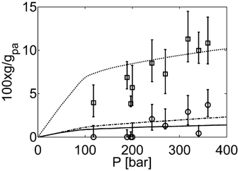
Calculated solubility of CO2 (dotted line) and VDF (continuous line) in amorphous domains of PVDF at T = 50 °C. Composition in supercritical phase: VDF/CO2 = 40:60 wt%. Values of the SL parameters are reported in Table 1 and 2. The curve of VDF solubility calculated using the SL parameter values adopted by Mueller et al.16 is also shown (dash-dotted line). Experimental data for CO2 (□) and VDF (○) from Galia et al.39
3.2. Kinetic Parameters: Continuous Phase
3.2.1. Initiation
According to Charpentier et al.,41 the initiator dissociation rate constant was assumed independent of pressure.  = 3.4 × 10⁻⁵ s−1 and initiator efficiency ψsc = 0.6 were used for DEPDC in scCO2 at T = 323 K.41, 42
3.2.2. Propagation and Termination
 ((31))
| Entry | [VDF] + [HFP] | fHFP,0 | [DEPDC] | Time | Xw | P0 |  |
 |
PDI |
|---|---|---|---|---|---|---|---|---|---|
| [mol · L−1] | [mol%] | [10−3 mol · L−1] | [min] | [%] | [MPa] | [mol%] | [kg · mol−1] | ||
| 1a) | 5.4 | 0 | 5.5 | 38 | 5.3 | 37.3 | 0 | 76.1 | 2.7 |
| 2a) | 4.3 | 6.1 | 5.3 | 60 | 5.5 | 29.4 | 1.5 | 51.3 | 1.9 |
| 3a) | 3.6 | 19.9 | 5.6 | 120 | 6.7 | 27.5 | 6.6 | 41.7 | 1.8 |
| 4b) | 5.8 | 28.6 | 6.9 | 30 | 4.3 | 40.0 | 9.4 | 66.9 | 1.7 |
| 5a) | 5.6 | 29.9 | 6.9 | 30 | 4.5 | 40.3 | 10.2 | 66.6 | 1.5 |
| 6b) | 5.4 | 30.5 | 12.4 | 55 | 6.5 | 37.6 | 10.0 | 53.4 | 1.5 |
| 7a) | 5.1 | 20.5 | 5.4 | 60 | 6.2 | 39.6 | 6.3 | 85.2 | 2.0 |
| 8b) | 5.5 | 21.5 | 5.4 | 60 | 8.7 | 39.6 | 6.7 | 74.3 | 2.7 |
| 9a) | 6.2 | 43.3 | 5.5 | 180 | 12.3 | 38.2 | 15.7 | 83.3 | 1.8 |
| 10a) | 9.3 | 47.7 | 5.5 | 180 | 12.4 | 39.2 | 18.6 | 129.3 | 2.4 |
- a) With surfactant;
- b) without surfactant.
 = 3000 L · mol−1 · s−1 (typical value; cf. Mueller et al.16), the values of the remaining kinetic parameters,
  and
and  , can be estimated from the measured number-average molecular weights. When termination occurs only by combination the following equation applies:44
 ((32))
 ((33))
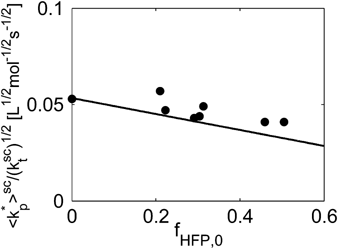
Using the experimental data collected at very low monomer conversion (Table 3), Equation 32 was used to estimate the values of the ratio  . Such values are shown in Figure 3 as a function of monomer feed composition for reactions carried out at initial pressures between P = 380 and 400 bar (symbols). In the same figure, the predicted values of the same quantity (see Appendix A) are plotted as continuous line. Using the ratio value at fHFP,0 = 0, i.e., in the PVDF case, and the typical value of
  mentioned above, the rate coefficient of bimolecular termination in supercritical phase was estimated as
  = 3.2 × 10⁹ L · mol−1 · s−1. Since it is well known that HFP is much less reactive than VDF, the cross propagation rate coefficient
  was constrained to be smaller than for the VDF homopolymerization (
 ≤
≤  ). Given this constraint, the best agreement which could be achieved with the experimental data is the one shown in Figure 3, obtained by setting the cross propagation coefficient
  equal to
  . The slight underestimation of the calculated values for the copolymer case can be due at least to two reasons: (i) experimental inaccuracies of the measured molecular weights from gel permeation chromatography (GPC) due to tailing at high molecular weight in the MWDs (cf. Costa et al.18); (ii) the experimental termination rate constant could be a (decreasing) function of the copolymer composition. On the other hand, the general agreement between calculated and experimental values is quite good and the approximation of composition-independent
  was retained. The values of the rate constants so far determined were considered valid at pressure of P = 400 bar.
 ((34))
 = 0 (as found by Charpentier et al.41) one obtains:
 ((35))
 ((36))
Equation 36 was used to estimate the activation volume of the propagation step from available low conversion experimental data.14 Using a typical value of  = 15 × 10−6 m3 · mol−1,16, 44
  = −76 × 10−6 m3 · mol−1 was calculated.
3.3. Kinetic Parameters: Dispersed (pa) Phase
3.3.1. Diffusion Coefficients
 ((37))
 are the weight fractions of the different species in phase i (i = sc or pa). In Equation 37, ρ*,
  are the SL characteristic densities of the pure component (indicated by the subscript) and of the mixture, while ρi is the density of phase i. For the generic component c with molecular weight MWc* of its “jumping unit”, ξA/c represents the ratio of the molar volumes of the monomer A and of the jumping unit of c:
 ((38))
 ((39))
Such value was estimated in order to provide reasonable predictions of diffusion coefficient of VDF in CO2-swollen PVDF: at 50 °C, under the operative conditions of Table 4 entry 1, the order of magnitude of  was about 10−9 dm2 · s−1, thus consistent with the range of experimental values of low-MW species in PVDF.49
| Entry | [VDF] + [HFP] | fHFP,0 | [DEPDC] |
|---|---|---|---|
| [mol · L−1] | [%] | [10−3 mol · L−1] | |
| 1 | 5.5 | 0.0 | 5.5 |
| 2 | 5.5 | 15.2 | 5.5 |
| 3 | 5.4 | 21.1 | 5.4 |
| 4 | 5.6 | 29.0 | 6.6 |
| 5 | 6.2 | 43.3 | 5.5 |
| 6 | 3.1 | 0.0 | 5.0 |
Equation 37 has been applied to both the polymer pa-phase and the continuous sc-phase. Notably, the values of most parameters are those previously estimated describing the phase behavior of the system. Accordingly, experimental values of the transport properties of the polymer-rich phase involved in the conventional VD-FV equation (cf. Keramopoulos and Kiparissides,46 Mueller et al.,16) are not needed any more: this represents a major step forward in the direction of simplifying the parameter evaluation process.
 ((40))
 is the average diffusion coefficient of the monomers
 ((41))
Note that, in the case under examination, we have found that the copolymer composition exhibits a very limited drift. Moreover, the composition of the copolymer produced in each phase is practically the same.18 Therefore, the cumulative composition of the entire copolymer is used in Equation 41 instead of the instantaneous composition in phase i.
3.3.2. Radical Interphase Transport
 ((42))
 are the (molar) partition and diffusion coefficients in phase i of radicals of length n, respectively. The radical partition coefficient is defined as:
 ((43))
 ((44))
 ((45))
 ((46))
The number of particles to be used in Equation 46, Np, was estimated from scanning electron microscopy (SEM) pictures. Such estimates were affected by the largely different particle morphologies. Dispersion reactions at fHFP,0 = 0–0.3 produced µm sized particles,18 with average particle concentration of Np/VR = 9.74 × 10¹³ L−1. Precipitation reactions at 0 < fHFP,0 < 0.3 produced irregularly shaped particles of average size 2–3 times larger,18 and therefore with particle concentrations about 10–30 times smaller. Accordingly, a particle concentration 20 times smaller was assumed for precipitation reactions leading to Np/VR = 4.87 × 10¹² L−1. Finally, in all reactions producing irregular and compact structures (precipitations at fHFP,0 = 0 and reactions with fHFP,0 > 0.4; Costa et al.18) we set a value of particle concentration arbitrarily small and equal to Np/VR = 9.74 × 10¹⁰ L−1, that is three order of magnitude smaller than the value used for dispersions providing µm sized spherical particles. Such choice is justified by the experimental observation that VDF precipitations produce aggregates at least ten times larger than the particles produced in dispersion reactions (cf. VDF precipitations in Charpentier et al.51, and VDF dispersions in Mueller et al.20)
3.3.3. Initiator Decomposition
 ((47))
3.3.4. Propagation and Termination
 ((48))
 ((49))
 and
and  are the self-diffusion coefficients in the pa-phase of the growing chains of length n and l, respectively. In Equation 48 and 49, the first term reflects the reactivity among radicals in the absence of diffusion limitations (i.e., that determined for the continuous phase), whose effect is accounted for in the second term. More details about physical meaning and derivation of Equation 48 and 49 are available in the cited literature.
 ((50))
The reliability of Equation 50 was tested using known values of the parameters a, σ, and ρ*: for example for MMA, using  = 1074 g · L−1,48 Equation 50 provides σMMA = aMMA = 0.67 nm, a value very close to those reported in the literature (aMMA = 0.69 nm and σMMA = 0.585 nm; Russell et al.53). For the system under examination, σVDF = 0.55 nm and σHFP = 0.61 nm have been estimated; being the two values similar, a single average value a = σ = 0.58 nm was used in all simulations.
3.3.5. Chain Transfer to Polymer
 ((52))
 has been introduced as a factor in Equation 52 because we assumed that only H atoms, present in the VDF units only, can be extracted by growing radicals. Apostolo et al.56 estimated a value of α = 3 × 10⁻⁵ for the emulsion copolymerization of VDF and HFP at T = 85 °C. Since there is evidence that temperature promotes branching formation,57 the value to be used to simulate reactions at T = 50 °C should be smaller. Accordingly, we set α = 10−6.
3.3.6. Tuning of Remaining Parameters
In this paragraph, the evaluation of all model parameters whose a priori prediction or estimation was not possible is discussed.
Let us consider the case of VDF homopolymerization first. In this case, all information related to monomer and radical solubility are available, by setting θ = 1 only the value of the entanglement spacing, jc,0, remains to be evaluated. Such value was determined by comparison of the experimental and calculated MWD of a single VDF dispersion polymerization, whose recipe is provided in Table 4 entry 1. Under these conditions, the large number of µm-sized polymer particles provided large interphase area and the polymerization occurred mainly in the dispersed phase. The resulting experimental MWD was broad but monomodal (cf. Figure 4a). The MWDs calculated by the model when using jc,0 = 50 and jc,0 = 200 (typical upper and lower limiting values of jc,0 as reported by Buback et al.55), are shown in Figure 4b as dashed and continuous lines, respectively. In both cases the model predictions underestimate the distribution broadening in the low-MW region. Decreasing jc,0 values result in reduced termination rate constants (cf. Equation 49 and 51) thus shifting the whole MWD toward higher MW and increasing the disagreement in the low-MW region (dashed vs. continuous line). As a result, the largest value of the entanglement spacing, jc,0 = 200, was selected as best value and kept constant in all simulations.
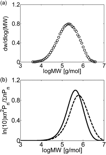
(a) Experimental MWD of PVDF obtained in a dispersion polymerization at VDF conversion of Xw = 41%. (b) Effect of chain transfer to polymer and entanglement spacing on MWD: jc0 = 200 (continuous line), jc0 = 50 (dashed line). Recipe in Table 4 entry 1.
Let us now consider the copolymer case. The monomer/copolymer interaction parameters, ηA/pol and ζA/pol, mainly affecting monomer partitioning between the sc and pa phase, and the radical partition coefficient, mn, affecting the radical transport rate (Equation 24, 25, 42), have to be evaluated as a function of the system composition. Indeed, several experimental evidences suggest that the thermodynamics of the system is heavily affected by the HFP content in the copolymer and by the composition of the fluid phase: the solubility of CO2 in PVDF is much smaller than in poly[VDF78-co-HFP22] (Supporting Information), the cloud point pressure of PVDF in CO2 is much larger than that of poly[VDF78-co-HFP22]29 and the solubility of the copolymer in the continuous phase is heavily affected by its HFP content.29, 58 Due to the difficulty of theoretically account for all these effects, a simplified approach aimed to minimize the number of adjustable parameters has been adopted, as detailed in the following.
To model monomer partitioning, ηA/pol was set to zero (like in the case of CO2), and ζVDF/pol was used as the only fitting parameter. The remaining parameter ζHFP/pol was adjusted to obtain the same instantaneous composition of the monomers in the two phases according to experimental results described elsewhere.18 Therefore, just one thermodynamic parameter was actually fitted (ζVDF/pol).
About the radical partitioning, the same mn values estimated for VDF homopolymerization were used. The effect of system composition on transport rates was accounted for through the adjustable quantity θ, the multiplying factor of the mass transport term in Equation 24 and 25. Accordingly, θ < 1 implies slower radical interphase transport compared to the PVDF case and vice versa.
Summarizing, two parameters only have to be determined by direct fitting of copolymer MWDs, θ and ζVDF/pol. Therefore, before comparing the model predictions to the experimental data, it is worth to analyze their impact on the model results in terms of MWD. At low conversion (Figure 5a), increasing θ from 0.1 (continuous line) to 1 (dashed line) at constant ζVDF/pol results in the disappearance of the mode at high molecular weight in the MWD. The larger amount of radicals transported into the pa-phase results in more polymer  at smaller chain length, and the two modes merge. On the contrary, larger monomer concentration in the pa-phase (decreasing ζVDF/pol) at constant θ = 0.1 (dotted line vs. continuous line), results in more polymer
  with larger molecular weight. Therefore, because of the opposite effect the two parameters have on the amount and molecular weight of the copolymer produced in pa-phase (cf. Figure 5b), θ and ζVDF/pol can be unambiguously tuned in order to match amount and location of the experimentally observed high-MW tail or mode in the MWDs using reactions carried out at low conversion. Such parameter evaluation was performed for the reactions carried out at fHFP,0 = 0.21 and fHFP,0 = 0.29 (Table 4 entries 3 and 4). In both cases, θ = 0.1 was estimated as best value. Such value was then used in all simulations at fHFP > 0.
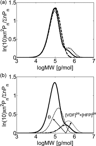
Calculated MWDs for low conversion VDF–HFP precipitation copolymerizations (recipe in Table 3, entry 4; at Xw = 4%). (a) Complete MWDs with: ζVDF/pol = 0.29 and θ = 0.1 (continuous line); ζVDF/pol = 0.25 and θ = 0.1 (dotted line); ζVDF/pol = 0.29 and θ = 1 (dashed line). (b) Complete MWDs with ζVDF/pol = 0.29 and θ = 0.1 (continuous line) and mode of chains produced in polymer phase (dash-dotted line). Also shown are the polymer phase contributions to the MWD for ζVDF/pol = 0.25 and constant θ = 0.1 (thin-dotted line); ζVDF/pol = 0.29 and constant θ = 1 (thin-dashed line). The arrows indicate the effect on the mode produced in the polymer phase when the monomer concentration in the pa-phase (dotted line) or the rate of radical transport (dashed line) increases.
Finally, the monomer partitioning and the corresponding values of ζA/pol (inset) are shown in Figure 6. At increasing HFP content in the monomer mixture, and therefore in the produced copolymer, the solubility of the monomers in the sc phase increases. The specific values of ζVDF/pol used to simulate the copolymerization at different compositions (e.g., fHFP,0 = 0.15 and 0.43 in Table 4 entry 2 and 5) were determined by interpolation or extrapolation and they are shown as empty symbols in Figure 6.
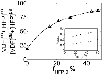
Calculated monomer partitioning between continuous (sc) and amorphous (pa) copolymer phase. T = 50 °C, P = 400 bar and [VDF]sc + [HFP]sc = 5.5 M. Inset: SL interaction parameters ζVDF/pol (○,•) and ζHFP/pol (□,▪) as a function of the monomer feed composition (the corresponding copolymer composition was calculated using the reactivity ratios rVDF = 3.6 and rHFP = 0).
4. Model Validation (Batch Reactions)
The effects of monomer feed composition, reaction time, interphase area, and pressure on the MWD of the final polymer are analyzed in the following in comparison with experimental results. Model was used in a genuinely predictive way using the parameter values estimated in the previous section and summarized in Table 5.
| Parameter | Value | Reference |
|---|---|---|
 |
1 | assumed |
 |
3.4 × 10⁻⁵ s−1 | |
| ψsc | 0.6 | |
| Xc | 0.521–3.554FHFP for FHFP < 0.147 |
determined from experimental results18 |
| 0 for FHFP > 0.147 | ||
| ρ0,pc | 1900 g · L−1 | |
| T0 | 298 K | |
| αpc | 0.0004 K−1 | |
| βpc | 1 × 10⁻¹⁰ Pa−1 | |
 |
3 000 L · mol−1 · s−1 (at 400 bar) |
typical value16 |
 |
 |
estimated from low-conversion data |
 |
3.6 | estimated from low-conversion data |
 |
0 L · mol−1 · s−1 | 15, 22, 28 |
 |
3.2 × 10⁹ L · mol−1 · s−1 (at 400 bar) | estimated from low-conversion data |
| α | 10−6 | this work; estimated |
 |
−76 × 10−6 m3 · mol−1 |
estimated from low-conversion data14 |
 |
15 × 10−6 m3 · mol−1 | typical value16, 44 |
| jc,0 | 200 | this work; estimated |
| a = σ | 0.58 nm | this work |
| Np/VR | 9.74 × 10¹³ L−1 for dispersions with 0 < fHFP,0 < 0.3; |
determined from experimental results18 |
| 4.87 × 10¹² L−1 for precipitations with 0 < fHFP,0 < 0.3; | ||
| 9.74 × 10¹⁰ L−1 for precipitations with fHFP,0 = 0 and reactions with fHFP,0 > 0.3 | ||
| D0 | 10−6 dm2 · s−1 |
typical value48 |
| γ | 0.2 |
typical value48 |
 |
0.6 | this work |
| mn | 0.404 × 10−0.04(n–11) for n ≤ 27; | |
| m27 × 10−0.2(n–27) for n > 27 | ||
| θ | 0.1 (for fHFP,0 > 0) | fitted from low-conversion data |
| δ | 0.5 µm | this work; assumed |
4.1. Effect of Monomer Composition
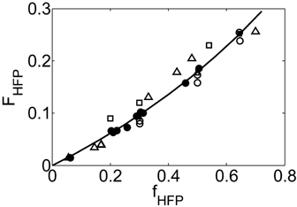
Let us consider first, copolymerization reactions carried out in the presence of surfactant, with 3 h reaction time (reaction recipes in Table 4 entries 1–5). Figure 7 and 8 show a good agreement between model (open symbols) and experimental data (filled symbols) in terms of conversion and copolymer composition, FHFP, as a function of the initial monomer feed composition, fHFP,0. For the same reactions, the experimental MWDs are shown as symbols in Figure 9-12, together with curves representing the model predictions. In all cases, the comparison is remarkably favorable. In particular, the gradual transition of the main MWD peak from high to low-MW region at increasing fHFP,0 is correctly predicted. From the model perspective, such transition indicates that the relevance of the dispersed phase as reaction locus progressively decreases when the starting monomer mixture is made richer in HFP. This behavior is explained by the lower radical transport rate compared to that of the homopolymer (θ < 1) and by the reduction of the monomer concentration (Figure 6) in the pa phase as fHFP,0 increases.
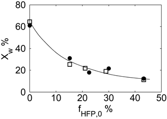
Experimental (•) and calculated (□, Table 4 entries 1–5) monomer conversion for VDF–HFP dispersion copolymerizations at 3 h reaction time. Line is a guide for the eye.
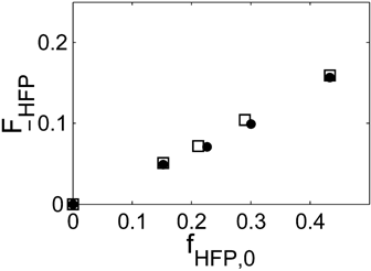
Experimental (•) and calculated (□, Table 4 entries 1–5) cumulative average copolymer composition,  , for VDF–HFP dispersion copolymerizations at 3 h reaction time.
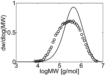
Experimental (○) and calculated (continuous line) MWD for VDF–HFP dispersion copolymerization at fHFP,0 = 0, reaction time of 3 h and conversion Xw = 61%, Table 4 entry 1.
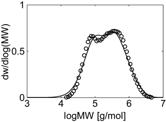
Experimental (○) and calculated (continuous line) MWD for VDF–HFP dispersion copolymerization at fHFP,0 = 0.15, reaction time of 3 h and conversion Xw = 31% (Table 4 entry 2).
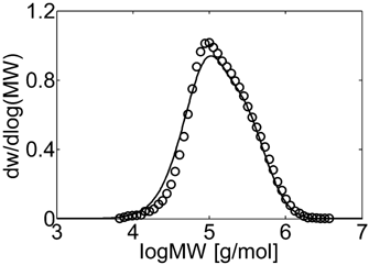
Experimental (○) and calculated (continuous line) MWD for VDF–HFP dispersion copolymerization at fHFP,0 = 0.3, reaction time of 3 h and conversion Xw = 22% (Table 4 entry 4).
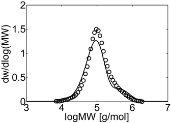
Experimental (○) and calculated (continuous line) MWD for VDF–HFP dispersion copolymerization at fHFP,0 = 0.4, reaction time of 3 h and conversion Xw = 12% (Table 4 entry 5).
4.2. Effect of Reaction Time and Interphase Area
The time evolution of the experimental MWDs for precipitation and dispersion copolymerization are shown in Figure 13a and 14a at an intermediate value of composition (fHFP,0 = 0.2), for which experimental data at small (precipitation) and large (dispersion) interphase areas but similar conversions and reaction times are available.18 At this HFP concentration in the reacting mixture, the solubility of the monomers in the dispersed phase is limited but still non-negligible. Accordingly, Figure 13a shows that for precipitation at small conversion, with a low amount of polymer present in the reactor, the lower molecular weight peak prevails against the high molecular weight shoulder in the MWD. Therefore, the homogeneous phase is the dominant reaction locus. On the other hand, at increasing reaction time and polymer hold-up, a distinct second peak becomes evident in the MWD, and the contribution of the polymer phase as reaction locus progressively increases, as clearly indicated by the relative increase of this second peak with time. Such MWD evolution with time was already observed for the precipitation of VDF.16 In the case of the dispersion reactions (Figure 14a), such evolution is similar but, because of the enhanced radical transport, the high-MW peak becomes the dominant one quickly, and the MWD at larger reaction time is still broad but monomodal. All these features are well predicted by the kinetic model, whose results are shown in Figure 13b and 14b. Even the drift of average composition is well captured (Figure 15). Note that having imposed equal monomer composition in the two phases, the calculated curves of copolymer composition for precipitation and dispersion reactions are identical.
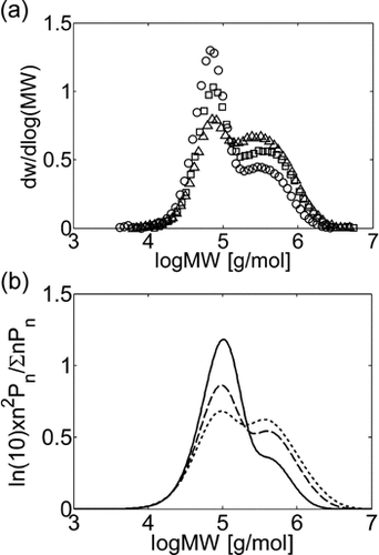
Experimental (a) and calculated (b) MWDs for VDF–HFP precipitation copolymerizations in scCO2 at fHFP,0 = 0.2, P0 = 380–400 bar and different conversion values: Xw = 9% (○, continuous line), Xw = 24% (□, dashed line), Xw = 42% (Δ, dashed line). Recipe in Table 5 entry 3.
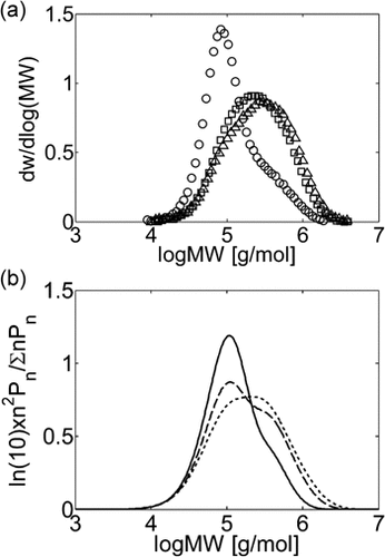
Experimental (a) and calculated (b) MWDs for VDF–HFP dispersion copolymerizations in scCO2 at fHFP,0 = 0.2, P0 = 380–400 bar and different conversion values: Xw = 6% (○, continuous line), Xw = 18% (□, dashed line), Xw = 36% (Δ, dashed line). Recipe in Table 5 entry 3.
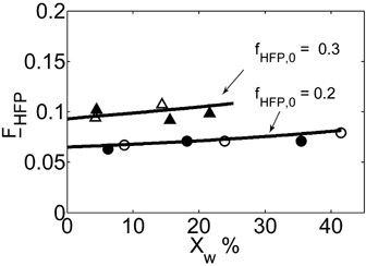
Experimental copolymer composition vs. conversion for VDF–HFP copolymerizations carried out at two different monomer feed compositions by precipitation (open symbols) and dispersion technique (filled symbols). The calculated curves for the two different reaction regimes are superimposed. Recipes in Table 4 entries 3, 4.
4.3. Effect of Pressure
In a previous contribution on VDF precipitation reactions, Mueller et al.16 showed that pressure enhances the reaction rate, and slightly shifts the whole bimodal MWDs toward larger MWs. The same authors showed that when using a value of  = −0.025 L · mol−1, that is a typical value for the activation volume of the propagation rate constant of many monomers, these effects were quite underestimated. In this work, a larger value of
  = −0.076 L · mol−1 was determined from experimental VDF–HFP precipitation data.14 Excellent predictions of the pressure effect on conversion and MWDs for VDF precipitations have been obtained, as shown in Figure 16 and 17, respectively. The enhanced reaction rates as well as the production of longer polymer chains at increasing pressure are quantitatively well reproduced. Therefore, despite the estimated
  is larger than typical literature values, the good agreement supports the reliability of such value for VDF-based copolymerization in scCO2. A possible explanation of such apparent overestimation might be the large variation of the solvent properties with pressure under supercritical conditions, as previously observed by other investigators.59-61
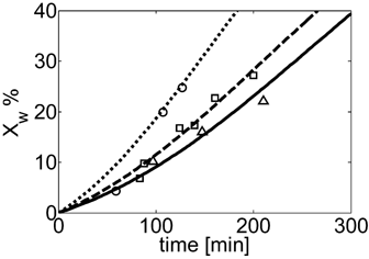
Conversion vs. time profiles for VDF precipitation polymerization in scCO2 at different initial pressure: P0 = 133 bar (Δ, continuous line), 204 bar (□, dashed line), 332 bar (○, dashed line). Curves represent model predictions. Recipes in Table 4 entry 8.
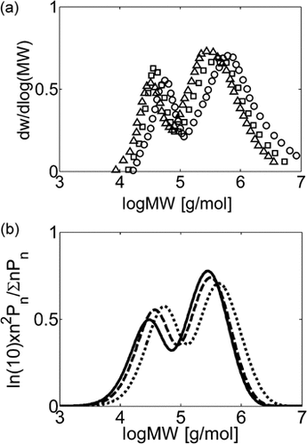
Effect of Pressure on experimental (a) and calculated (b) MWDs at Xw = 25% for VDF precipitation polymerization in scCO2: P0 = 133 bar (Δ, continuous line), 204 bar (□, dashed line), 332 bar (○, dashed line). Recipe in Table 4 entry 6.
5. Modeling of CSTR Data
A final check of the model reliability and of the parameter values was performed by comparing model predictions with experimental data from independent sources.
Saraf et al.17 and Ahmed et al.14 carried out precipitation reactions in scCO2 using a CSTR with monomer mixture feed composition fHFP = 0 at T = 75 °C and P = 277 bar, and fHFP = 0.265 at T = 40 °C and P = 400 bar, respectively. In order to account for the different temperature, the values of the three rate coefficients in the supercritical phase only (initiator dissociation constant,  , homopropagation rate constant
  and the termination rate constant,
  ) were changed as detailed in Appendix B. All the remaining model parameters were kept constant and equal to those reported in Table 5. The experimental MWDs for VDF precipitation polymerizations at increasing monomer concentration are shown in Figure 18a. At small monomer concentration ([VDF] < 1 M) a negligible amount of monomer is absorbed inside the small amount of formed polymer. The continuous phase is the dominant reaction locus and the resulting MWD is narrow and monomodal. At increasing monomer concentration, first a shoulder and then a well defined peak at high MW appear. The model predictions, shown in Figure 18b, reproduce this behavior quite closely: the appearance and location of the second peak are well predicted and only the very long tail at the largest monomer concentration is underestimated. The same qualitative picture was observed for VDF–HFP precipitation copolymerizations at increasing monomer concentration, as shown in Figure 19a. However, because of the preferential partitioning of the monomers into the continuous phase compared to the homopolymer case, the polymerization rate in the dispersed phase is smaller. As a consequence, at increasing monomer concentration a long tail first and then a pronounced shoulder in the MWD appeared instead of a well defined second mode. Qualitatively, the model results (Figure 19b) compare again well with the experimental data, even if the amount of polymer produced in the dispersed phase and the extension of the tail were underestimated.
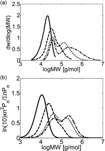
MWD at different monomer feed concentration for VDF precipitation polymerization in CSTR. τ = 21 min, T = 75 °C, P = 277 bar. (a) Experimental MWDs (Saraf et al.17) and (b) model predictions at [VDF]in = 0.78 (continuous line), 1.68 (dashed line), 2.82 (dotted line), and 3.53 mol · L−1 (dash-dotted line).
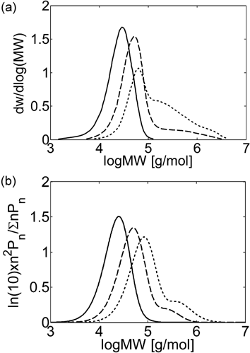
MWDs at different monomer concentration for precipitation copolymerization in CSTR. τ = 20 min, T = 40 °C, P = 400 bar. (a) Experimental results (Ahmed et al.14) and (b) model predictions at fHFP,in = 0.265 and [VDF]in + [HFP]in = 1.96 (continuous line), 3.92 (dashed line), 6.53 mol · L−1 (dotted line).
6. Comments
6.1. Bimodality in the MWDs
The prediction ability of the proposed 2-loci model in terms of occurrence, location, and relative amount of the larger-MW mode in the complete MWD was remarkable in all cases (cf. Figure 10, 13, and 17). This is especially true when considering that the interface area, Ap, was not taken as an adjustable parameter as previously done in the case of VDF precipitation polymerization.16 Nevertheless, the model nicely predicted the monomer concentration effect on VDF surfactant free polymerization (Figure 18), as well as the effect of the increase of interphase area when, adding an effective surfactant, dispersion copolymerizations were performed, as shown in Figure 13 and 14. The fair comparison with the experimental MWDs is a further confirmation of a mechanistic picture involving two phases as possible reaction loci.
6.2. Monomer Partitioning
Ahmed et al.62 speculated that because of the preferential partitioning of the monomers in the scCO2-rich phase and the resulting poor solubility of the monomers in the polymer phase, the propagation of radicals in the polymer phase should occur under starved conditions, and therefore with negligible polymerization rate. With this respect, two points must be addressed. First, the monomer solubility in the polymer phase is small but not negligible. For example, in the first minutes of reaction, the model predicts VDF concentration in the amorphous polymer phase of about 0.3 mol · L−1 at the conditions given in Table 4 entry 1. Second, while the propagation rate constant is almost unaffected by diffusion limitations (Equation 48), the termination rate constant in pa-phase is orders of magnitudes smaller than that in sc phase, as shown in Figure 20. Therefore, such very low  value counterbalances the low monomer solubility and makes possible a fast polymerization rate in pa phase.
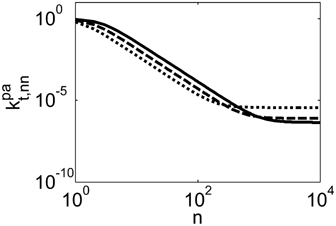
Ratio between termination rate constant in the pa and in the sc phase calculated for dispersion polymerizations (computed at 10% monomer conversion). Recipes in Table 1 entry 1 (dotted line), entry 3 (dashed line) and entry 5 (continuous line).
About the values of the interaction parameters used for VDF/PVDF, note that they differ from those reported by Mueller et al.16 and Galia et al.39. The reason is that different sets of data were used to determine both the pure component and binary SL interaction parameters. Nevertheless, from the model perspective, the exact value of the interaction parameters is not crucial. Indeed, the important point is to describe correctly the monomer sorption in the polymer matrix. In Figure 1, experimental sorption data of VDF in PVDF are compared with profiles calculated with the SL EOS using parameters determined by Mueller et al.16 (dash-dotted curve) and those used in this study (continuous line). It can be observed that the two profiles are quite similar and both match with acceptable agreement the experimental data.
7. Conclusion
The heterogeneous copolymerization of VDF and HFP in supercritical carbon dioxide (scCO2) occurs both in the continuous and in the dispersed polymer-rich phase. This mechanistic view is supported by the observation that the MWD of the produced copolymer is heavily affected by the interphase area of the polymer phase, Ap: bimodal or monomodal MWDs are obtained under precipitation (lower Ap) or dispersion polymerization conditions (higher Ap), respectively.
Accordingly, in this work a heterogeneous copolymerization model consistent with the 2-loci schematization is developed as an evolution of a previous homopolymerization model.16 It is accounting for radical transport between the phases, diffusion limitations affecting propagation and termination, as well as chain length dependent rate constant for the termination reactions occurring in the polymer-rich, dispersed phase. As expected, the resulting model involves a very large number of kinetic parameters, whose evaluation is indeed asking for a major effort. This is especially true because we are dealing with multiple monomers and heterogeneous systems. Therefore, a specific parameter evaluation strategy has been used in order to estimate most of them a priori using independent experimental or theoretical information, while minimizing the number of parameters estimated by direct fitting of the experimental data. For example, the LFV was applied to evaluate the diffusion coefficients both in the continuous as well as in the dispersed phase, thus largely reducing the number of parameters characterizing the polymer phase compared to traditional approaches.
The model well describes the effect of reaction time, pressure, interphase area, and monomer feed composition on conversion and MWD. In particular, the occurrence and location of the bimodality in the MWDs are well predicted.
At increasing reaction time and interphase area the relative abundance of the higher molecular weight mode in the MWD progressively increases because of enhanced radical transport in the polymer phase.
Vice versa, at increasing HFP content in the monomer feed mixture, the role of the polymer phase as reaction locus becomes less important and, as a consequence, the relative abundance of the higher molecular weight mode in the MWD progressively decreases. This is interpreted as due to preferential partitioning of radicals and monomers in the supercritical phase at increasing HFP content in the feed and in the resulting copolymer, thus causing reduced radical transport rate and reactivity in the polymer phase.
Nomenclature
-
- []
-
Concentration [mol · L−1]
-
- a
-
Root-mean end-to-end distance divided by the square root of the number of monomer units in a polymer chain [dm]
-
- Ap
-
Interphase area [dm2]
-
- A, B
-
Generic monomer (VDF or HFP) [mol]
-
- c
-
Subscript, generic component (VDF, HFP, CO2, or amorphous polymer)
-
 ,
, 
-
Self-diffusion coefficient of the generic monomer A, and of a growing radical of length l [dm2 · s−1]
-
- D0
-
Pre-exponential coefficient for the self-diffusion coefficients [dm2 · s−1]
-

-
Monomer A mole fraction (based on monomers only) in phase i
-
 , FA
, FA -
Copolymer average composition (cumulative and instantaneous)
-
- i = sc, pa, pc
-
Superscript indicating supercritical phase, amorphous polymer phase, and crystalline polymer phase, respectively
-
- in
-
Subscript, denoting reactor inlet conditions (in CSTR)
-
- I
-
Initiator (DEPDC) [mol]
-
- jc,0
-
Pure polymer entanglement spacing
-

-
Initiator decomposition rate constant in phase i [s−1]
-
- kf
-
Transfer to polymer rate constant [L · (mol · s)−1]
-

-
Average propagation rate constant in phase i [L · (mol · s)−1]
-

-
Propagation rate constant for reaction between A-terminated radical and B monomer unit in phase i [L · (mol · s)−1]
-

-
Average propagation rate constant for reaction between a radical and an A monomer unit in phase i [L · (mol · s)–1]
-

-
Value of the average propagation rate constant time monomer concentration in phase i [s−1]
-

-
Termination rate constant between radicals of length n and l in phase i [L · (mol · s)−1]
-
- Kn
-
Global transport coefficient referred to the sc phase for radicals of length n [dm · s−1]
-
- mc, mn
-
Partition coefficient for the generic component c, and for radicals of chain length n (expressed as molar concentration in the sc phase divided by the molar concentration in the pa-phase)
-
- mix
-
Subscript denoting mixture property
-

-
Molecular weight of the jumping unit for species c [g · mol−1]
-
- MW,

- MW,
-
Molecular weight and number-average molecular weight [g · mol−1]
-
- MWD
-
Molecular weight distribution
-
- NAV
-
Avogadro constant [mol−1]
-
- Nc
-
Number of components
-
- Np
-
Number of polymer particles
-
- n, l
-
Index denoting chain length
-
- P
-
Pressure [Pa]
-

-
Characteristic pressure of component c [Pa]
-

-
Amount of dead chains of length n, formed by a termination event occurred in phase i [mol]
-
- pol
-
Polymer or copolymer (subscript, or superscript)
-
- rA
-
Reactivity ratio for monomer A
-
- ru
-
Copolymer repeating unit
-
- rnl
-
Minimum distance at which radicals instantaneously terminate [dm]
-
- R
-
Universal gas constant [J · (mol · K)−1]
-
- Ri,
 ,
, 

- Ri,
-
Radicals, radicals of length n, and radicals of length n whose active site is an A unit, respectively. All referred to phase i [mol]
-
- sc
-
Number of mers for the component c
-
- t
-
Time [s]
-
- T
-
Temperature [K]
-

-
Characteristic temperature of c component [K]
-
- T0
-
Reference temperature [K]
-
- VR, Vi
-
Reactor and phase i volume [L]
-

-
Characteristic volume [L · mol−1]
-
- vp
-
Volume of a polymer particle [L]
-
- Xcr
-
Degree of crystallinity (defined on a mass basis)
-
- Xnucl
-
Monomer mass conversion at which nucleation occurs instantaneously
-
- Xw
-
Monomer mass conversion
Greek Letters
-
- α
-
Ratio between transfer and propagation rate constant
-
- αpc
-
Thermal expansion coefficient for the crystalline polymer [K−1]
-
- βpc
-
Compressibility of the crystalline polymer [Pa−1]
-
- δ
-
Thickness of the boundary layer [m]
-
- δn,1
-
Kronecker delta function (equal to 1 for n = 1, 0 otherwise)
-
- ΔV*
-
Activation volume [m3 · mol−1]
-
- φc
-
Close-packed volume fraction for component c
-
- ψi
-
Initiator efficiency in phase i
-

-
Chemical potential of component c in phase i [J · mol−1]
-
- λj,

- λj,
-
Moment of the jth-order for dead chains, and dead chains formed in phase i, respectively [mol]
-

-
Characteristic energy [J · mol−1]
-

-
Weight fraction of component c in phase I
-
- σ
-
Monomer size [dm]
-
- ξA/c
-
Ratio between the jumping unit molar volumes of the generic monomer A and component c
-
- γ
-
Overlap factor
-
- ρi
-
Density of phase i [g · L−1]
-

-
Characteristic density [g · L−1]
-
- ρ0,pc
-
Density of the crystalline copolymer, at reference conditions [g · L−1]
-
- θ
-
Effective transport rate parameter
-
- ηcj, ζcj
-
SL interaction parameters between component c and j
-
- τ
-
Residence time (in CSTR) [s]
Acknowledgements
The financial support of Università di Palermo is gratefully acknowledged.
Appendix A: Long-Chain Approximation (LCA)
 ((A1))
 ((A2))
 ((A3))
 ((A4))
 ((A5))
 ((A6))
 ((A7))
 ((A8))
 ((A9))
 ((A10))
 ((A11))
 ((A12))
 ((A13))
 ((A14))
 ((A15))
 ((A16))
Appendix B: Determination of Rate Constants for CSTR Reactions
Regarding the initiator dissociation constants, Charpentier et al.41 measured  = 9.9 × 10⁻⁴ s−1 for DEPDC at T = 75 °C, and Ahmed et al.14 indicated
  = 4 × 10⁻⁴ s−1 for perfluorobutyryl peroxide (PBP) at T = 40 °C. Such values have been used to model CSTR data obtained at the corresponding temperatures.
For copolymerization reactions, conducted at temperature quite close to the one at which kinetic parameters were determined (T = 40 °C), we kept constant the termination rate constant and updated only  (at the reference pressure of 400 bar), in order to correctly position the calculated MWD of the polymer corresponding to the reaction occurred in the continuous phase. The same procedure could not be applied to the case of VDF precipitation polymerizations because we found it would have lead to an unrealistically high value of
  > 8000 L · mol−1 · s−1. Therefore, we applied an Arrhenius type temperature dependency for
  with activation energy of 15 000 J · mol−1, and the MW mode peak in the MWD corresponding to the polymer formed in the continuous phase was correctly located by tuning of
  . The obtained values at the reference pressure of P = 400 bar are given in Table B1. Note that, in all cases, we assumed
  =
=  ,
,  = (
= ( )/3.6,
  = 0, and all cross termination constants equal.
| Entry | T |  |
 |
 |
|---|---|---|---|---|
| [°C] | [s−1] | [L · mol · s−1] | [L · mol · s−1] | |
| 1 | 75 | 9.9 × 10⁻⁴ | 4 479 | 8.87 × 10⁸ |
| 2 | 40 | 4 × 10⁻⁴ | 4 403 | 3.2 × 10⁹ |
 , reported in Table B2 (last column) well compare with the experimental ones, determined by:44
 ((B1))
 . Experimental values determined using Equation B1 and then, to be compared with model values, corrected at the same reference pressure of P = 400 bar using Equation 34.


