Characterisation of multiple conducting permeable objects in metal detection by polarizability tensors

3.1 Multiple homogeneous objects that are sufficiently well spaced

We consider N homogenous-conducting permeable objects of the form   †with Lipschitz boundaries where, for the nth object, B⁽ⁿ⁾ denotes a corresponding unit sized object located at the origin, α⁽ⁿ⁾ denotes the object's size, and z⁽ⁿ⁾ the object's translation from the origin. The union of all objects is where we use a bold subscript α to denote the possibility that each object in the collection can have a different size. We also employ the same notation for the fields E_α and H_α, which satisfy 1. An illustration of a typical configuration is shown in Figure 1. In this figure, there are N = 3 objects, which are the spheres , n = 1,2,3, where, for the nth object, α⁽ⁿ⁾ is its size (here its radius), and z⁽ⁿ⁾ is its translation from the origin. In the presented case, B = B⁽¹⁾ = B⁽²⁾ = B⁽³⁾ is a unit sphere located at the origin although, in practice, the objects do not need to have the same shape.

We generalise the definitions of μ_α and σ_α previously stated in Section 2 to

where and set and for n = 1,…,N. We introduce and set , and require that the parameters of the inclusions be such that

which implies that ν⁽ⁿ⁾ = O(1).

The task is then to provide a low-cost description of (H_α − H₀)(x) for x away from B_α. This is accomplished through the following result.

Theorem 3.1.For the arrangement B_α of N homogeneous conducting permeable objects with and parameters such that ν⁽ⁿ⁾ = O(1) , the perturbed magnetic field at positions x away from B_α satisfies

(5)

where

uniformly in x in any compact set away from B_α. The coefficients of the complex symmetric MPTs , n = 1,…,N, can be computed independently for each of the objects α⁽ⁿ⁾B⁽ⁿ⁾ using the expressions

(6a)

(6b)

These, in turn, rely on the vectoral solutions , k = 1,2,3, to the transmission problem

(7a)

(7b)

(7c)

(7d)

(7e)

where , Γ⁽ⁿ⁾: = ∂B⁽ⁿ⁾ and ξ⁽ⁿ⁾ is measured from an origin chosen to be in B⁽ⁿ⁾.

3.2 Single inhomogeneous object

In this case, describes a single object comprised of N constitute parts, , such that there is a single common size parameter α, the configuration B contains the origin, and z is a single translation, as illustrated in Figure 2. Notice that for the inhomogeneous case, we use rather than (B_α)⁽ⁿ⁾ as α is the same for all n, and we revert to the use of nonbold α subscripts for the fields E_α and H_α, which satisfy 1.

The material parameters of the constitute parts of the object B_α are

where , and we drop the subscript α on μ and σ when considering the object B. We redefine with the same requirements on as before.

The task is then to provide a low-cost description of (H_α − H₀)(x) for x away from B_α. This is accomplished through the following result.

Theorem 3.3.For an inhomogeneous object, B_α = αB+z made up of N constitute parts with parameters such that the perturbed magnetic field at positions x away from B_α satisfies

(8)

where

uniformly in x in any compact set away from B_α. The coefficients of the complex symmetric MPT are given by

(9a)

(9b)

which, in turn, rely on the vectoral solutions θ_k, k = 1,2,3, to the transmission problem

(10a)

(10b)

(10c)

(10d)

where ξ is measured from the centre of B and, in this case, .

4.1 Elimination of the current source

Recall from the previous research1 that

and the weak solution for the interaction field is: Find such that

where (·,·)_Ω denotes the standard L² inner product over Ω. In a departure from the previous study,1 we have, for multiple objects, that

Noting that the weak solution for the background field is: Find such that

we can write: Find such that

which eliminates the current source. We also obtain that

(11)

4.2 Energy estimates

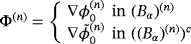
In the existing work,1 a vector field F(x) was introduced such that its curl is equal to the first two terms of Taylor's series expansion of ∇ × E₀ about z for |x−z|→0 for the case of a single object B_α. This was possible as the current source J₀ is supported away from the object and so is analytic where the expansion is applied. We extend this to the multiple object case by requiring that J₀ be supported away from B_α and introduce the following for n = 1,…,N

so that

In other words, ∇ × F⁽ⁿ⁾(x) is the first two terms in a Taylor series of iωμ₀H₀(x) about z⁽ⁿ⁾ as |x−z⁽ⁿ⁾|→0 and so

(12)

where here and in the following C denotes a generic constant unless otherwise indicated.

The introduction of F⁽ⁿ⁾(x) motivates the introduction of the following problem: Find such that

(13)

where . By the addition of such problems, we have

(14)

where , in (B_α)⁽ⁿ⁾ and in (B_α)⁽ⁿ⁾.

We also remark that associated with 13 is the strong form

(15a)

(15b)

(15c)

(15d)

(15e)

(15f)

which follows from using

Lemma 4.2.For objects (B_α)⁽ⁿ⁾ and (B_α)^(m) with n ≠ m, we have that

Proof.Introducing , which, without loss of generality, we assume the origin to be in B⁽ⁿ⁾. We set and so . Note that satisfies

(16a)

(16b)

(16c)

(16d)

(16e)

(16f)

From the above, we have that for sufficiently large |ξ⁽ⁿ⁾| and so we estimate that for the same case. Thus, for m ≠ n,

where we have used .□

Corollary 4.3.Given the description , we are free to configure B⁽ⁿ⁾ in different ways provided that the origin lies at a point in B⁽ⁿ⁾ (similarly with ) . Thus, |z^(m) − z⁽ⁿ⁾| will be smallest when the origin lies in the boundaries of the objects, as illustrated in Figure 4. Requiring that then Lemma 4.2 implies that

The following Lemma extends Ammari et al's Lemma 3.21 to the case of N multiple objects, when they are sufficiently well spaced.

Lemma 4.4.Provided that , there exists a constant C such that

for n = 1,…,N where μ_r,max := max_{n = 1,…,N}μ_*⁽ⁿ⁾/ μ₀.

Proof.We start by proceeding along the lines presented in1 and introduce where

with being the solution of an exterior problem in an analogous way to in the previous study.1 Using 11 and 14 (and after multiplying by μ₀), we can deduce that

(17)

where and in (B_α)⁽ⁿ⁾. Choosing v=E_α − E₀ − (w_α + Φ_α) then we have that

Also, by application of the Cauchy-Schwartz inequality, we can check that

(18)

where

(19)

(20)

(21)

To bound A₁ and A₂ we have used 12,

(22)

and applied similar arguments to the previous study.1 The terms A₃ does not appear in the single object case and dictates the minimum spacing for which the bound holds. Requiring that and applying Corollary 4.3 then

(23)

Using 19-20, and 23 in 18 we find that

and by additionally using , this completes the proof.□

By recalling the definition of stated in Lemma 4.2, Ammari's et al's Theorem 3.11 in the case of multiple sufficiently well spaced objects becomes

Theorem 4.5.Provided that , there exists a constant C such that

The expressions for α⁽ⁿ⁾F⁽ⁿ⁾(z⁽ⁿ⁾ + α⁽ⁿ⁾ξ⁽ⁿ⁾) and are obtained by extending in an obvious way the expressions in given in (3.13) and (3.14) in the previous study1 where the latter is now written in terms of as well as where and satisfy the transmission problems

(24a)

(24b)

(24c)

(24d)

(24e)

(24f)

and

(25a)

(25b)

(25c)

(25d)

(25e)

(25f)

The properties of and are analogues to the single object case presented in the previous research.1

4.3 Integral representation formulae

Repeating the proof of Lemma 3.3 in the previous study1 for the multiple object case, it extends in an obvious way to

Lemma 4.6.Let be the union of N bounded domains each with Lipschitz boundaries whose outer normal is n. For any satisfying ∇ × ∇×E=0, ∇·E=0 in , we have, for any

In a similar way, repeating the proof of their Lemma 3.4 for multiple objects it extends in an obvious way to

Lemma 4.7.Let . Then for

4.4 Asymptotic formulae

Ammari et al's Theorem 3.21 presents the leading order term in asymptotic expansion for (H_α − H₀)(x) for a single inclusion B_α as α→0. In the case of multiple objects that are sufficiently well spaced, this extends to

Theorem 4.8.For a collection of N objects such that ν⁽ⁿ⁾ is order one, α⁽ⁿ⁾ is small and then for x away from B_α we have

(26)

where is the solution of (24) and

(27)

uniformly in x in any compact set away from B_α.

Proof.The proof uses as its starting point Lemma 4.7 and considers each object (B_α)⁽ⁿ⁾ in turn. It applies very similar arguments to the proof of Ammari et al's Theorem 3.21 except Theorem 4.5 is used in place of their Theorem 3.1, 22 is used in place of their (3.6) and note that

(28)

by integration by parts. Furthermore, to recover the negative sign in the first term in 26, we have used

(29)

as α⁽ⁿ⁾→0. Theorem 3.21 mistakingly uses as α→0, which leads to the wrong sign in their first term, as previously reported for the single homogenous object case.2□

5.1 Elimination of the current source

The results presented in Section 4.1 hold also in the case when the object is inhomogeneous except the subscript α is replaced by α.

5.2 Energy estimates

For an inhomogeneous object, we proceed along similar lines1 and introduce a single vector field F(x) whose curl is such that it is equal to the first two terms of a Taylor series of iωμ₀H₀(x) expanded about z as |x−z|→0

so that

(30)

The introduction of F(x) motivates the introduction of the following problem: Find such that

(31)

The following Lemma extends Ammari et al's Lemma 3.21 to the case of an inhomogeneous object.

Lemma 5.1.For an inhomogeneous object B_α , there exists a constant C such that

(32)

(33)

for m = 1,…,N.

Proof.Here we introduce where

with being the solution of an exterior problem in an analogous way to.1 Then, by writing

and proceeding with similar steps,1 where B_α is replaced by B_α, we have

(34)

for m = 1,…,N and

Finally, we use and , which holds for n = 1,…,N.□

Introducing, so that we find that w₀(ξ) satisfies

(35a)

(35b)

(35c)

(35d)

(35e)

(35f)

where, for an inhomogeneous object, .

In this case, Ammari et al's Theorem 3.11 becomes

Theorem 5.2.There exists a constant C such that

for m = 1,…,N, which holds for an inhomogeneous object B_α.

The expressions for αF(z+αξ) and w₀(ξ) are identical to Ammari et al's (3.13) and (3.14)1 where θ_i(ξ) and ψ_ij(ξ) now satisfy the transmission problems

(36a)

(36b)

(36c)

(36d)

(36e)

(36f)

and

(37a)

(37b)

(37c)

(37d)

(37e)

(37f)

The properties of θ_i(ξ) and ψ_ij(ξ) are analogues to the homogeneous object case presented in the previous study.1

5.3 Integral representation formulae

The integral representation formulae presented in Section 4.3 only require (B_α)⁽ⁿ⁾ to be replaced by and H_α to be replaced by H_α for an inhomogeneous object.

5.4 Asymptotic formulae

Ammari et al's Theorem 3.21 presents the leading order term in asymptotic expansion for (H_α − H₀)(x) for a single homogenous inclusion B_α = αB+z as α→0. In the case of an inhomogeneous inclusion, this becomes

Theorem 5.3.For an inhomogeneous object B_α such that ν⁽ⁿ⁾ is order one and α is small then for x away from B_α, we have

(38)

where θ_i is the solution of (36) and

(39)

uniformly in x in any compact set away from B_α.

Proof.The proof uses as its starting point Lemma 4.7 and considers each region in turn. It applies similar arguments to the proof of Ammari et al's Theorem 3.21 except that our Theorem 5.2 is used in place of their Theorem 3.1 and our 34 instead of their (3.6). Furthermore, note that by summing contributions, we have that

(40)

by application of integration by parts and, in a similar manner to the proof of Theorem 4.8, we use

(41)

to give the correct negative sign in the first term of 38.□

6.1 Numerical illustration of asymptotic formulae for (H_α − H₀)(x)

To illustrate the results in Theorems 3.1 and 3.3, comparisons of (H_α − H₀)(x)  ‡will be undertaken with a finite element method (FEM) solver19 for multiple objects and for inhomogeneous objects. We first show comparisons for two spheres, then comparisons for two tetrahedra followed by comparisons for an inhomogeneous parallelepiped.

6.1.1 Two spheres

We first consider the situation of two spheres (B_α)⁽¹⁾ and (B_α)⁽²⁾. These objects are defined as

which means that the radii of the objects are α⁽¹⁾ and α⁽²⁾, respectively. Setting B = B⁽¹⁾ = B⁽²⁾ to be a sphere of unit radius placed at the origin then

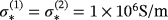
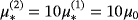
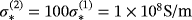
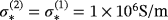
are the location of the centroids of the physical objects and , respectively. Thus, the objects (B_α)⁽ⁿ⁾, n = 1,2, are centered about the origin with . The material properties of the spheres are , , we use ω = 133.5rad/s and the object sizes are chosen as α = α⁽¹⁾ = α⁽²⁾ = 0.01m and hence , independent of their separation, which will be used in Theorem 3.1. For closely spaced objects, we expect Theorem 3.3 to be applicable, and in this case,we set

and z=0. Note that in this case, must be recomputed for each new d.

Comparisons of (H_α − H₀)(x) obtained from the asymptotic formulae 5 and 8 in Theorems 3.1 and 3.3 as well as a full FEM solution are made in Figure 5 for d = 0.2 and d = 2 along three different coordinates axes. To ensure the tensor coefficients were calculated accurately, a p = 3 edge element discretisation and an unstructured mesh of 6581 tetrahedra are used for computing and meshes of 8950, and 11940 unstructured tetrahedral elements are used for computing for d = 0.2 and d = 2, respectively. In addition, curved elements with a quadratic geometry resolution are used for representing the curved surfaces of the spheres. For these, and all subsequent examples, the artificial truncation boundary was set to be 100|B|. To ensure an accurate representation of (H_α − H₀)(x) for the FEM solver, the same discretisation, suitably scaled, as used for is employed.

For the closely spaced objects, with d = 0.2, we observe good agreement between Theorem 3.3 and the FEM solution in Figure 5, with all three results tending to the same result for sufficiently large |x|. The improvement for larger |x| is expected as the asymptotic formulae 5 and 8 are valid for x away from B_α≡B_α. For objects positioned further apart, with d = 2, we observe that the agreement between Theorem 3.1 and the FEM solution is best. This agrees with what our theory predicts, since, for d = 2, and so this theorem applies.

6.1.2 Two tetrahedra

Next, we consider the case of two tetrahedra where the physical objects (B_α)⁽¹⁾ and (B_α)⁽²⁾ are chosen as the tetrahedra with vertices , , , , and , , , , scaled by α⁽¹⁾ and α⁽²⁾ respectively. Thus, the objects (B_α)⁽ⁿ⁾, n = 1,2, are centered about the origin with and we determine B⁽ⁿ⁾ from by setting

such that the centroid of B⁽ⁿ⁾ lies at the origin. A typical illustration of the two tetrahedra is shown in Figure 6. The sizes and materials of (B_α)⁽¹⁾ and (B_α)⁽²⁾ are both the same, as in the previous section, but due to their different shapes, although the MPTs are independent of d. However, note that (B_α)⁽²⁾ = α⁽²⁾R^x((B_α)⁽¹⁾)/α⁽¹⁾ and B⁽²⁾ = M^x(B⁽¹⁾), where

and since α = α⁽¹⁾ = α⁽²⁾ the tensor coefficients transform as

(42)

For , we instead choose B⁽¹⁾ = (B_α)⁽¹⁾/α⁽¹⁾, B⁽²⁾ = (B_α)⁽²⁾/α⁽²⁾ and set z=0.

Comparisons of (H_α − H₀)(x) for this case are made in Figure 7 for d = 0.2 and d = 2 along three different coordinates axes. To ensure the tensor coefficients are calculated accurately, a p = 3 edge element discretisation and unstructured meshes of 15617 and 15488 tetrahedra are used for computing and , § respectively, and meshes of 15837 and 22045 unstructured tetrahedral elements are used for computing for d = 0.2 and d = 2, respectively. To ensure an accurate representation of (H_α − H₀)(x) for the FEM solver, the same mesh, suitably scaled, as used for is employed with p=6.

As in Section 6.1.1, we observe good agreement between Theorem 3.3 and the FEM solution for the closely spaced objects in Figure 7, with all three results tending to the same result for sufficiently large |x|. For objects positioned further apart, with d = 2, we observe that the agreement between Theorem 3.1 and the FEM solution is again best, which again agrees with what our theory predicts, since, for d = 2, , and so this theorem applies.

6.1.3 Inhomogeneous parallelepiped

In this section, an inhomogeneous parallelepiped with

is considered. The material parameters of (B_α)⁽¹⁾ and (B_α)⁽²⁾ are , , and , , respectively.

Comparisons of (H_α − H₀)(x) obtained from using the asymptotic expansion 8 in Theorem 3.3 and a full FEM solution are made in Figure 8 along three different coordinates axes. To ensure the tensor coefficients are calculated accurately, a p = 3 edge element discretisation and an unstructured mesh of 13121 tetrahedra are used for computing . To ensure an accurate representation of (H_α − H₀)(x) for the FEM solver, the same mesh, suitably scaled, as used for is employed with p=5. We observe a good agreement between Theorem 3.3 and the FEM solution for sufficiently large |x|.

6.2 Frequency spectra

The frequency response of the coefficients of for a range of single homogeneous objects has been presented in existing studies3, 4 where the real part was observed to be sigmoid with respect to and the imaginary part had a distinctive single maxima. Rather than consider the coefficients, it is in fact better to split in to the real part and an imaginary part , which are both real symmetric rank 2 tensors, and to compute the eigenvalues of these. Indeed, many of the objects previously considered had rotational and/or reflection symmetries such that the eigenvalues coincide with the real and imaginary parts of the diagonal coefficients.

A theoretical investigation of and , where corresponds to the real symmetric rank 2 tensor describing the limiting response in the case of ω→0, and agrees with the Póyla-Szegö tensor for a homogenous permeable object, has been undertaken.20 In this, we prove results on the eigenvalues of these tensors.

Now, considering for an inhomogeneous object B_α, the coefficients of are given by

(43)

where

(44a)

(44b)

(44c)

(44d)

(44e)

and we have shown that for , the eigenvalues of and have the properties and (this also applies to a homogenous objects where B_α reduces to B_α).20

To illustrate how the behaviour of and changes for an inhomogeneous object, we consider the geometry of the parallelepiped described in Section 6.1.3 placed at the origin so that with α = 0.01m. Note that, although and have different properties, the object B still reflectional symmetries in the e₁ and e₃ axes and a π/2 rotational symmetry about e₁ so that the independent coefficients of are and (and hence , are the independent coefficients of and , are the independent coefficients of ). In Figure 9, we show the computed results for and for the case where and , and in Figure 10, we show the corresponding result for and . For this, we use similar discretisations to those stated previously. In the former case, vanishes but not in the latter case.

We observe, in Figure 9, that although , i = 1,… ,3 are still monotonically decreasing with , it is no longer sigmoid for an inhomogeneous object with varying σ and constant μ and has multiple nonstationary inflection points. Furthermore, rather than a single maxima, , i = 1,… ,3 has two distinct local maxima. However, the results shown in Figure 10 illustrate for an inhomogeneous object with varying μ and constant σ, , i = 1,… ,3, that the behaviour is quite different, and in this case, , i = 1,…,3 is still sigmoid and the curves for , i = 1,…,3 still have a single maxima. In the limiting case of ω→0, , i = 1,…,3 and, for the latter case with a contrast in μ, the behaviour is as shown in Figure 11, which is quite different to a homogenous object of the same size.

To investigate the behaviour of inhomogeneous objects still further, we next consider the inhomogeneous parallelepiped with

and α = 0.01m. To compute , an unstructured mesh of 15 109 tetrahedral elements is generated and p = 4 elements employed. The independent coefficients of are again and .

In Figure 12, we show and for the case where and , and in Figure 13, we show the corresponding result for and . In the former case, vanishes, but not in the latter case.

We observe, in Figure 12, that , i = 1,…,3 is still monotonically decreasing with multiple nonstationary points of inflection, and , i = 1,…,3 now has three distinct local maxima. In Figure 13, we see that , i = 1,…,3 is sigmoid, and , i = 1,…,3 has only a single maxima. Unlike Figure 11, we see in Figure 14 that the low frequency response of λ_i(Re(M[αB])), i = 1,…,3 are different. This is probably due to the fact that the chosen contrasts in μ imply that one of the three cubes no longer has a dominant effect over the other two.

6.3 Object localisation

The approach described by Ammari, Chen, Chen, Volkov, and Wang6 for a single object localisation using multistatic measurements simplifies given our object characterisation in terms of rank 2 MPT for a single homogenous object and also easily extends to inhomogeneous and multiple objects. Following their study,6 we assume that there are K receivers at locations r^(k), k = 1,…,K, which are associated with small measurement coils with dipole moment q, and L sources at locations s^(ℓ), ℓ = 1,…,L, which are associated with small exciting coils each with dipole moment p. Then, by measuring the field perturbation described by Theorem 3.1 for N_target = N objects in the direction q, this gives rise to the k, ℓth entry of the multistatic response matrix as

where, for the purpose of the following, we arrange the coefficients of the rank 2 tensors as 3 × 3 matrices. ¶ Assuming that the data is corrupted by measurement noise and is sampled using Hadamard's technique, as in the previous study,6 then the MSR matrix can be written in the form

where and W is a K × L matrix with independent and identical Gaussian entries with zero mean and unit variance, and S_noise is a positive constant. In addition, U is a matrix of size K × 3N_target

and U⁽ⁿ⁾ is an K × 3 matrix

The matrix is of size 3N_target × 3N_target and is block diagonal in the form

and the matrix V is of dimension 3N_target × L with

where V⁽ⁿ⁾ is the 3 × L matrix

(45)

Proceeding in a similar manner to the previous research,6 and defining the linear operator as

(46)

then, by dropping the higher order term, the MSR matrix can be approximated as

The MUSIC algorithm can then be used to localise the location of the multiple arbitrary shaped targets by using the same imaging functional as proposed in the previous study6

(47)

where P is the orthogonal projection onto the right null space of .

We explore this through the following experiment. We simulate excitations and measurements taken at regular intervals on the plane [ − 1,1] × [ − 1,1] × {0} such that L = K = 256. The dipole moments are chosen as p=q=e₃ so that the plane of all measurement, and excitation coils are parallel to this horizontal surface. With these measurements, the location identification of a coin of radius 0.01125m and thickness 3.15 × 10⁻³m with and and a tetrahedron with vertices (5.77 × 10⁻³,0,0)m, ( − 2.88,5,0) × 10⁻³m, ( − 2.88, − 5,0) × 10^− 3m and (0,0, − 8.16 × 10⁻³)m and material properties and will be considered. The true locations of these objects are assumed to be and , respectively. To perform the imaging, noise is added to the simulated A₀ to create A, and the image functional I_MU is evaluated for different positions z^s. To do this, we compute where W_S are the first 3N singular vectors of A, which are chosen based on the magnitudes of the singular values and thereby allows us to also predict the number of objects N present.

We first consider location identification at a frequency f = 1 × 10⁵Hz, which is close to the resonance peaks for the two objects, and consider the singular values of A₀ and A in Figure 15. At this frequency, S_n(A₀), n = 1,2,3 are associated with the coin and S_n(A₀), n = 4,5,6 with the tetrahedron. Without noise, A = A₀ and the six physical singular values are clearly distinguished, but, by considering a noise level of 1% so that S_noise = 0.01S₁(A₀), it is no longer possible to distinguish S_n(A), n = 4,5,6 from the noisy singular values. On the other hand, by setting S_noise = 0.01S₄(A₀), or even S_noise = 0.1S₄(A₀), we can distinguish all 6 singular values from the noise. This means that with S_noise = 0.01S₁(A₀) we expect to only locate the coin, but with S_noise = 0.01S₄(A₀),0.1S₄(A₀) we expect to find both objects. This is confirmed in Figure 16 where we plot I_MU on the plane −0.5e₃. We observe that for S_noise = 0.01S₁(A₀), we can only locate the coin, for S_noise = 0.01S₄(A₀) we can locate both the coin and the tetrahedron and even by increasing the noise level to 10% and setting S_noise = 0.1S₄(A₀) both objects can still be identified. On the other hand, choosing the frequency f = 132Hz, such that S_n(A₀), n = 1,2,3 are associated with the tetrahedron and S_n(A₀), n = 4,5,6 with the coin, Figure 17 shows that the phenomena is reversed, and with a 10% noise level and S_noise = 0.1S₄(A₀), only the tetrahedron can be identified at this frequency.

6.4 Object identification

A dictionary-based classification technique for individual object identification has been proposed by Ammari et al6 and this easily extends to the identification of multiple inhomogeneous objects. We propose a slight variation on that proposed by Ammari et al, which uses the eigenvalues of the real and imaginary parts of the MPT as a classifier as opposed to its singular values at a range of frequencies. The motivation for this is the richness of the frequency spectra of the eigenvalues, as shown in Section 6.2 and that it provides an increased number of values to classify each object. We also propose a strategy in which objects are put in to canonical form before forming the dictionary. The algorithm comprises of two stages as described below.

6.4.1 Offline stage

In the offline stage, given a set of N_candidate candidate objects (which can include both homogenous and inhomogeneous objects), we put them in canonical form , i = 1,…,N_candidate by ensuring that the origin for ξ⁽ⁱ⁾ in B⁽ⁱ⁾ coincides with the centre of mass of B⁽ⁱ⁾ and the object's size α⁽ⁱ⁾ is chosen such that   #where in the case of a homogenous object and corresponds to the Póyla-Szegö tensor as well as being the characterisation for σ_∗ = 0 for this object. ∥ In the case of an object with homogenous materials, the coefficients of are computed by solving the transmission problem (7) using FEM and then applying (6), and in the case of an inhomogeneous object, (10) and (9) are used. In each case, the eigenvalues and are obtained for a range of frequencies ω_j and

forms the ith element of the dictionary

6.4.2 Online stage

In an extension to the previous research,6 the MPT coefficients for each of the targets (T_α)⁽ⁱ⁾, i = 1,…,N_target can be recovered from the same data used to identify the number and locations of objects. Although, to do so, it is important to ensure that the dipole moments of the coils are chosen such that all the 6N_target coefficients can be recovered from the measured data.4 The coefficients are then the solution of the least squares problem

which is repeated for j = 1,…,N_ω.

Then, for each target (T_α)⁽ⁱ⁾, we determine

and find the closest match to within the dictionary .6 Notice the target could also be inhomogeneous in which case (T_α)⁽ⁱ⁾ is replaced by .

6.4.3 Numerical example

As a challenging object identification example, we consider a dictionary consisting of parallelepipeds described in Section 6.2, which consist of either two regions with or three regions with , and vary the material properties according to the descriptions previously described. We also consider the limiting case where the two (three) regions have the same parameters. The dictionary for these objects is generated according to the off-line stage with ω ∈ 2π(2,300,4 × 10³,5 × 10⁴,2 × 10⁵)rad/s, arbitrarily chosen over the frequency spectrum.

For the online stage, take , i = 1,2, j = 1,…,N_ω = 5 to be given by considering targets where R is an arbitrary rotation and adding noise. In Figure 18, we illustrate the algorithms ability to differentiate between these similar objects. The red bars indicate the predicated classification, which is correct for the examples presented (it was also found to be correct for the cases of the other parallelepipeds). We can observe that greatest similarity in terms of the classification is between the two homogeneous parallelepipeds and between the two parallelepipeds with contrasting σ, and in each case, the classification becomes more challenging as the noise level is increased.

By increasing the number of frequencies considered so that N_ω = 7 with ω ∈ 2π(2,300,4 × 10³,5 × 10⁴,2 × 10⁵,3 × 10⁶,4 × 10⁷)rad/s, we see in Figure 19 that the certainty of the classification is improved for both noise levels.