1 Introduction

Polypropylene (PP) is one of the most commonly used thermoplastics for industrial applications because of its high formability,^[1] which means that it can easily be molded into a wide range of shapes. Additionally, PP shows a high resistance to a variety of degradation processes such as oxidation and chemical attack, and thus is frequently used in corrosive environments.^[2] However, these factors also give rise to one of the greatest drawbacks of PP which is the environmental impacts from its waste.^[3] It accounts for 16% of global plastic production,^[4] of which only 1% was recycled in 2015, which means that most of that waste is put into landfill or incinerated.^[5] A much better alternative would be to recycle a higher proportion of PP in use whilst still retaining a significant fraction of the properties of the virgin material.

In thermomechanical recycling processes, PP experiences high temperature and shear stresses when reheated and remolded. This degrades a number of its properties, such as tensile and impact strengths, Young's modulus, and durability. Although the mechanism for the degradation depends on the recycling process, it is generally explained by the fact that free radicals are generated when PP is exposed to thermal energy or stress, causing chain scission and a decrease in molecular weight.^[6] To improve the mechanical properties of recycled PP, other polymers such as rubbers and elastomers are often mixed in with it.^[7-10] Another approach to increase its mechanical properties is by the introduction of physical or chemical crosslinks. For example, Kaewkuk et al. demonstrated that incorporating PP-g-MA and sisal fibers into native PP leads to an increase in the mechanical properties such as tensile strength and Young's modulus compared to the virgin polymer.^[11] The PP-g-MA can interact with the hydroxy groups of the fibers via its carboxyl groups, and its chains also defuse into PP, enhancing the interactions between the sisal fibers and PP matrix, and thus building physical crosslinks. Candia et al. also improved the Young's modulus and tensile strength of isotactic polypropylene (iPP) by chemically introducing crosslinks.^[12]

In addition to these conventional methods to introduce physical or chemical crosslinks, recent studies have developed techniques for producing dynamic covalent bonds, which form and break reversibly via external stimuli including heating and the addition of catalysts. Polymers with dynamic covalent bonds behave like thermosets except that they can be melted once they are exposed to a stimulus. This enables not only the control of polymer properties by changing the crosslink density, similarly to the conventional techniques, but also the capability to readily recycle the materials. Saed et al. have applied such methods to PP, showing that mechanical properties such as the tensile strength are affected by the bond density, and that the PP can be melted at a certain temperature by breaking of the bonds.^[13] In order to obtain polymers with desired properties by these approaches, the contribution of crosslink density to their mechanical properties must be well understood. Nevertheless, the mechanical properties of polymers are usually affected not only by crosslink density but also by other parameters such as crystallinity and molecular weight, which can be also changed by crosslink density.^[14] This makes it difficult to isolate the influence of crosslink density on mechanical properties in many cases.

In order to address this, some studies have employed computational methods such as molecular dynamics (MD) to investigate the effects of crosslink density on mechanical properties including tensile strength, fracture strain, and Young's modulus in various polymers.^{[15, 16]} However, although thermoset plastics obtained by a curing process, including epoxy resin, are often investigated by these techniques, there are relatively fewer studies focusing on crosslinked rubbers and polyolefins, such as PP. Since thermosetting plastics requiring a curing process usually start from small molecules, of order a few tens or hundreds of grams per mole, many computational techniques can model these despite their system-size limitations. As the curing progresses, although the molecules become larger, the molecular weight between crosslinks (M_c) is usually around several hundreds of grams per mole^[17] which is still sufficiently low to be reproduced by many theoretical methods. On the other hand, in crosslinked rubbers and polyolefins, where crosslinks are introduced into already formed polymer chains, M_c ranges more widely from a few hundreds to tens of thousands of grams per mole.^{[18, 19]} Some computational techniques such as the MD method have difficulty in simulating sufficiently large networks to examine the contribution of crosslink density on mechanical properties over such a wide range of densities. Regarding iPP, which we selected in this study among the three PP structures with different types of tacticity (isotactic, atactic, and syndiotactic PPs) due to its extensive usage (> 90%) in industry,^[20] its entanglement molecular weight (M_e) in its native state, without introduced crosslinks, is reported as around 6900  g mol⁻¹.^[21] The entanglement points in iPP cannot be disentangled during mechanical tests at a room temperature and thus behave like chemical crosslinks, playing a significant role in affecting the stress–strain behaviors.^[22] If the entanglement points are interpreted as permanent crosslinks, then M_c decreases from 6900  g mol⁻¹ as crosslinks are introduced, and therefore the changes in the mechanical properties in this range of crosslink density would be of most interest. However, it is still too computationally expensive for techniques such as all-atom MD to reproduce the iPP structures with a realistic range of crosslink densities and to carry out mechanical tests on them.

To overcome such length limitations, many coarse-grained techniques have been developed,^[23] and the dissipative particle dynamics (DPD) method is one of the most commonly employed techniques for many materials including polymers.^[24] In the DPD method, several atoms are grouped into a single particle which makes it possible to treat the system on a larger length scale. The standard DPD force field consists of three terms: the conservative, dissipative, and random forces.^{[25, 26]} The increased softness of these interactions enables us to employ a larger timestep and thus to achieve a larger time scale. As with other empirical methods, DPD simulation requires parameters for its interactions, and some optimization techniques have been suggested such as iterative Boltzmann inversion,^[27] force matching,^[28] and Green–Kubo formulae.^[29] Recently, Bayesian optimization has been applied to derive DPD parameters.^[30] It is related to force-matching techniques and optimizes DPD parameters to reproduce a reference trajectory obtained by an all-atom MD simulation. Compared to standard force-matching approaches, it has several advantages: 1) it provides time-averaged parameters and thus reaches more satisfactory optimization; 2) it is less likely to suffer from overfitting; and 3) the friction parameter for the dissipative force can be obtained simultaneously as well as those for other interactions. Thus, we have employed Bayesian optimization to derive DPD parameters for a coarse-grained model of amorphous iPP and then evaluated the mechanical properties of iPP structures with a realistic range of crosslink densities in DPD simulations.

In summary, this work aims at obtaining a better understanding of the contribution of crosslink density to mechanical properties such as the Young's modulus and ultimate strength in amorphous iPP structures with realistic crosslink densities using the DPD technique. Among three structures of PP with different types of tacticity, isotactic, atactic, and syndiotactic PPs, we selected isotactic PP (iPP) because, as mentioned above, it is the most commonly used in industry. Hereafter, we first explain the procedure used to build a coarse-grained model of iPP and optimize its DPD parameters. The computational workflow includes the following steps: an all-atom MD simulation to generate a reference trajectory, Bayesian optimization to obtain the DPD parameters, and validation of the coarse-grained iPP with the optimal parameters. Next, the coarse-grained model of iPP and the optimized parameters are applied to examine the influence of crosslink density on the mechanical properties. The protocol for changing the crosslink density and performing mechanical tests in DPD simulations are also provided. We then discuss the results of the stress–strain curves from iPP structures with different numbers of crosslinks, and relate the crosslink density to the mechanical properties such as the Young's modulus and ultimate strength.

2 Coarse-Grained Model Development

We employed Bayesian optimization to obtain DPD parameters for the coarse-grained iPP model.^[30] In this method, DPD parameters are derived that maximize the probability of reproducing the forces observed in a reference trajectory from an all-atom MD calculation. We first carried out an MD simulation to generate an all-atom trajectory. This was then converted to a coarse-grained model to be used as a reference trajectory for Bayesian optimization. Using this trajectory, the DPD parameters for coarse-grained iPP were optimized by Bayesian optimization. Next, DPD simulations were performed to validate the coarse-grained iPP with the optimal parameters by comparing its properties in the DPD simulations with those evaluated in MD simulations. The details of the procedure are described below.

2.2 Coarse-Graining Procedure

We then converted the all-atom trajectory into a coarse-grained expression. We grouped two repeat units into one bead. This produced three types of beads with different structures and masses (shown in Figure 1): two types are for the two repeat units at the ends of iPP (Bead1 and Bead3 in Figure 1), and the other is for those between the polymer ends (Bead2 in Figure 1). Both Bead1 and Bead3 consist of C₃H₇-C₃H₆ with a mass of 85.17 g mol⁻¹ despite their slightly different structures, while Bead2 has a structure of (C₃H₆)₂ with a mass of 84.16 g mol⁻¹. Although these beads have slightly different structures and masses, we used identical interaction parameters to describe them. Based on these definitions, we mapped the all-atom trajectory onto a coarse-grained one using bead representation for Bayesian optimization. Hereafter, we refer to this coarse-grained trajectory obtained by an all-atom MD simulation as a CGMD trajectory.

2.3 Parameterization

2.3.1 Functional Forms for Interactions

To evaluate the mechanical properties of iPP, the conservative non-bonded interactions were expressed by the LJ potential instead of the conventional DPD form consisting of only a repulsive force. Although the 12–6 LJ potential is commonly used for atomic systems, we employed the softer 4–2 LJ potential for the coarse-grained beads:

$$$$\begin{equation} V^{\rm nb}(r_{ij}) = {\begin{cases} 4 \epsilon {\left[ {\left(\frac{\sigma }{r_{ij}} \right)}^{4} - {\left(\frac{\sigma }{r_{ij}} \right)}^2 \right]} & {\left(r_{ij} < r_{\rm c} \right)} \\ 0 & {\left(r_{ij} \ge r_{\rm c} \right)} \end{cases}} \end{equation}$$$$(1)

where r_ij = |r_ij| = |r_i − r_j| is the distance between beads i and j, ϵ is the minimum energy at a distance of $$\sqrt {2} \sigma$$, σ is the distance at which the force changes its sign, and r_c is a cutoff distance. This is because the 12–6 LJ potential was too steep to reproduce the soft interactions between iPP beads in DPD simulations (see Section S1, Supporting Information). The weighting factors for 1–2, 1–3, and 1–4 neighboring beads were set to 0, 0.5, and 1, respectively.

For bonding interactions to connect iPP beads to their first neighbors, we combined two harmonic potentials switched at a threshold distance of r_b:

$$$$\begin{equation} {V}^{\rm bond}(r_{ij}) = {\begin{cases} k_{\rm b,1} {\left(r_{ij} - r_{0,1} \right)}^2 & {\left(r_{ij} < r_{\rm b} \right)} \\ k_{\rm b,2} {\left(r_{ij} - r_{0,2} \right)}^2 & {\left(r_{ij} \ge r_{\rm b} \right)} \end{cases}} \end{equation}$$$$(2)

where k_b,1 and k_b,2 are force constants, and r_0,1 and r_0,2 are reference bond distances. In the CGMD trajectory, the distribution of bond lengths shows two sharp peaks (shown in Figure 2b below), which cannot be reproduced using only a single harmonic potential. Hence, we employed two different harmonic potentials as shown in Equation (2), and we set r_b = 4.9 Å based on the position of the local minimum between two peaks in the distribution of bond length. On the other hand, this generated a discontinuous point of V^bond(r_ij) at the distance of r_b, as well as a discontinuous function of bond forces obtained by taking the derivative of the potential. In DPD simulations using LAMMPS, a function of bond force is used to compute forces exerted on bonds at each step, and thus this discontinuity can result in unexpected behavior of iPP beads and make the system unstable. To prevent this, the function for bond interactions was made continuous at r_b by smoothing the two profiles of bond forces obtained from the two harmonic potentials in Equation (2) in a region around r_b (see Section S2, Supporting Information). Furthermore, although a quartic bond potential, which is one of commonly used bond potentials, has two local minima and thus results in two peaks in the distribution of bond length, we found that these two different harmonic potentials provided a better distribution of bond length compared to the MD system and were therefore selected for the bond potential. The distances r_0,1 and r_0,2 were optimized during Bayesian optimization as well as the force constants of k_b,1 and k_b,2. ^[40]

Meanwhile, for bond bending interactions, we used a single harmonic potential:

$$$$\begin{equation} V^{\rm angle}(\theta _{ijk}) = k_{\rm a} {\left(\theta _{ijk} - \theta _0 \right)}^2 \end{equation}$$$$(3)

where k_a and θ₀ are a force constant and the reference bond angle between beads i, j, and k.

Regarding the dissipative and random forces, the standard DPD expressions were employed:^[26]

$$$$\begin{equation} f_{ij}^{\rm D} = - \gamma w_{ij}^2 {\left({\mathbf {e}}_{ij} \cdot {\mathbf {v}}_{ij} \right)} {\mathbf {e}}_{ij} \end{equation}$$$$(4)

$$$$\begin{equation} f_{ij}^{\rm R} = \sigma w_{ij} \theta {\mathbf {e}}_{ij} \end{equation}$$$$(5)

where γ is a friction parameter, e_ij = r_ij/r_ij is the unit vector connecting beads i and j, v_ij = v_i − v_j is the relative velocity of beads i and j, σ is a noise parameter satisfying $$\sigma = \sqrt {2 \gamma k_{\rm B} T}$$, θ is a Gaussian random number with zero mean and unit variance, and w_ij is a weight function given by

$$$$\begin{equation} w_{ij} = {\begin{cases} {\left(1- \frac{r_{ij}}{r_{\rm c}} \right)} & {\left(r_{ij} < r_{\rm c} \right)} \\ 0 & {\left(r_{ij} \ge r_{\rm c} \right)} \end{cases}} \end{equation}$$$$(6)

2.3.2 Bayesian Optimization

The parameters for the DPD interactions given above were fitted by Bayesian optimization.^[30] When the conservative force can be expressed by a linear combination of DPD parameters, the contribution of the conservative force at time t, $$\mathbf {F}_t^{\rm C}$$, is written as

$$$$\begin{equation} \mathbf {F}_t^{\rm C} = \mathbf {A}_t \mathbf {x}^{\rm C}, \end{equation}$$$$(7)

where A_t is a matrix that depends only on the bead positions at time t in the CGMD trajectory and is calculated from Equations (1), (2), and (3), and x^C is the parameter set to be optimized for the conservative interaction defined in these equations. The dissipative force, $$\mathbf {F}_t^{\rm D}$$, is given by

$$$$\begin{equation} \mathbf {F}_t^{\rm D} = - \gamma \mathbf {B}_t \mathbf {V}_t, \end{equation}$$$$(8)

where B_t is a symmetric matrix depending only on bead positions at time t as shown in Equation (4).

Using the A_t and B_t matrices defined in Equations (7) and (8), Bayesian optimization gives the optimal parameter set for the conservative force, $$\mathbf {\bar{x}}^{\rm C}$$:

$$$$\begin{equation} \mathbf {\bar{x}}^{\rm C} = {\left(\sum _t \mathbf {A}_t^* \mathbf {B}_t^{-1} \mathbf {A}_t \right)}^{-1} {\left(\sum _t \mathbf {A}_t^* \mathbf {B}_t^{-1} \mathbf {F}_t^{\rm ref} \right)}. \end{equation}$$$$(9)

where $$\mathbf {F}_t^{\rm ref}$$ is the reference force at time t obtained in the CGMD trajectory.^[30] In Bayesian optimization, the A_t and B_t matrices are calculated for each snapshot in a reference CGMD trajectory according to the bead positions and cutoff distance.

Bayesian optimization provides optimal parameters maximizing the probability to reproduce the forces observed in the CGMD trajectory. This implies that there can be three possible ways to reproduce the reference forces: the first is by using only repulsive forces, like the conventional DPD form of the conservative force, the second is by using only attractive forces, and the third is by using a mixture of both repulsive and attractive forces. To evaluate mechanical properties, we need both repulsive (short-range) and attractive (long-range) terms, which is why we chose the LJ potential. However, even when the LJ potential is employed, fixing a single cutoff distance during Bayesian optimization can result in undesirable solutions, in which either purely repulsive or purely attractive forces were found when reproducing the reference forces (see Section S3, Supporting Information).

To avoid these inappropriate optimizations, although the same cutoff distance is usually employed to compute the A_t and B_t matrices from each snapshot in a reference CGMD trajectory, we introduced two different cutoff distances: the first one (a larger cutoff distance of 21.5 Å) was used with a probability of 90%, and the second one (a shorter cutoff distance of 7.5 Å) was employed with a probability of 10%. The larger cutoff distance was determined to reproduce the density of iPP obtained in the CGMD trajectory by a DPD system (see Section S4, Supporting Information). This means that the two matrices were calculated based on the larger cutoff distance in 90% of the snapshots while the shorter cutoff distance was used in 10% of the snapshots. This is based on an assumption that the undesirable optimizations may be significantly affected by the cutoff distance because either only repulsive or attractive forces are employed to reproduce the reference forces. Therefore, using the shorter cutoff distance would work as a penalty to avoid inappropriate optimizations and enhance the probability to reach the targeted optimization. The Bayesian optimization process failed to reach a target solution where the reference forces were reproduced by a mixture of both repulsive and attractive forces even when taking into account volume fluctuations in the reference trajectory.^[30] Therefore, we employed this modified algorithm using two different cutoff distances to avoid inappropriate solutions. The DPD parameters optimized by Bayesian optimization are summarized in Table 1. These parameters are shown in real units instead of non-dimensional units, which are often used in DPD simulations, because they were obtained from a reference trajectory generated by an MD simulation using real units. Thus, in the following DPD simulations, real units were also employed. Although some of these interactions may be stronger than conventional DPD forces, we confirmed that the fluctuation-dissipation theorem was satisfied, and thus temperature was kept constant in the following DPD simulations.

Table 1. The optimized parameters for the interactions between iPP beads in DPD simulations.

Parameter	Optimized value	Unit
ϵ	0.20	kcal mol−1
σ	7.03	Å
kb,1	1.49	kcal mol−1Å−2
r0,1	4.78	Å
kb,2	4.83	kcal mol−1Å−2
r0,2	5.08	Å
ka	0.82	kcal mol−1
θ0	143.28	degree
γ	0.15	kcal fs mol−1Å−2

2.4 Validation

2.4.1 Structural Properties

To ensure that the coarse-grained model of iPP and the optimized DPD parameters accurately reproduce the system compared to the CGMD trajectory, we performed a DPD simulation using the optimal parameters in Table 1. We used the final snapshot in the MD simulation conducted to relax an all-atom expression of iPP in Section 2.1 to build an initial structure for a DPD simulation. We first converted it to a coarse-grained model and then duplicated it along the x-, y-, and z-directions to build an initial structure with 2³ (=8) times the volume of the original all-atom model. Next, using the initial structure, a DPD simulation employing the NpT ensemble was carried out with a timestep of 50 fs for 100 ns at 298 K. The cutoff distance was set to 21.5 Å, which was employed as the larger cutoff distance for Bayesian optimization. Structural parameters were averaged over the last 10 ns to be compared with those in the CGMD trajectory.

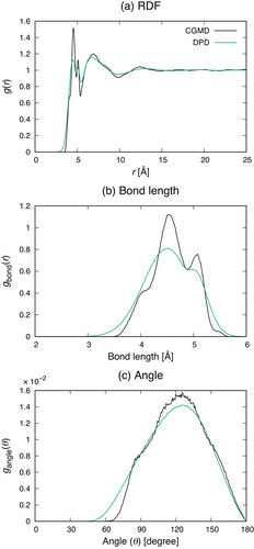
We first compared the radial distribution function (RDF) obtained in the DPD simulation with that evaluated from the CGMD trajectory (Figure 2a). This figure shows that the RDF obtained in the DPD simulation is in good agreement with that from the CGMD trajectory. Although the two peaks at about 5 Å in the system of DPD are not as sharp as those in the CGMD trajectory, due to the softness of interaction potential, their positions are consistent in both methods. Additionally, the broad peaks at around 7 Å are almost identical with each other.

Then, Figure 2b,c compare the bond and angle distributions in DPD simulations with those obtained in the CGMD trajectory. The bond distribution has sharp two peaks at about 4.5; 5.0Å, which correspond to the two peaks at the same positions in the RDF in Figure 2a. Similarly to the RDF, the two peaks in a DPD calculation are broader, but their positions are well reproduced. Additionally, the angle distributions are also in a good agreement with each other.

Next, as a property on a larger length scale, we compared radii of gyration between MD and DPD simulations. The MD simulation gave the value of 19.0 Å while the DPD method yields 20.4 Å. Although the radius of gyration was not directly taken as a targeted property when optimizing the DPD parameters, the value in the MD simulation was well reproduced by the DPD method.

2.4.2 Mechanical Properties

Furthermore, we carried out mechanical tests to obtain the stress–strain curve of iPP in MD and DPD simulations. In an MD simulation, we set the last snapshot in the MD simulation conducted to relax an amorphous iPP in Section 2.1 to an initial structure. In a DPD method, the last snapshot in the DPD calculation performed to evaluate the structural properties was used as an initial structure. We conducted three calculations in both methods to deform the structure of amorphous iPP along the x-, y-, and z-directions with an engineering strain rate of 1.0 × 10¹⁰ s⁻¹. During these simulations with the deformations imposed along the x-, y-, and z-axes, the xx-, yy-, and zz-components of the stress tensors were recorded respectively every 100 steps to obtain three stress–strain curves. They were smoothed by a moving average with 100 data points and then averaged over the three directions to obtain a stress–strain curve. Regarding the directions orthogonal to the applied stress direction, a pressure of 1 atm was applied.

Figure 3 shows the stress–strain curves and orientational order parameter as a function of true strain during the mechanical tests in MD and DPD simulations. Regarding the orientational order parameter, bond vectors between first neighboring beads were defined in the CGMD and DPD trajectories of the mechanical tests, and we calculated orientational order parameters P given by

$$$$\begin{equation} \left< P \right>= \frac{\left< 3 {\rm {cos}^2} \theta -1 \right>}{2}, \end{equation}$$$$(10)

where θ is an angle between bond vectors and the applied strain direction.

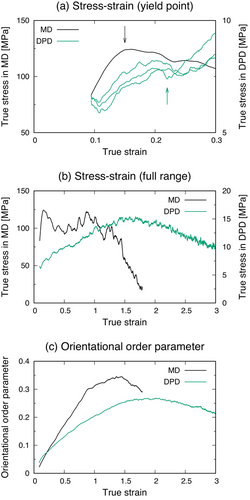
Looking at the stress–strain curves in Figure 3, the stress values for the DPD simulation are underestimated compared to those in the MD simulation, and thus the stress–strain curve in MD is shown with the first y-axis while those in DPD simulations are displayed with the second y-axis. This may be because the DPD parameters were optimized by the reference trajectory at an equilibrium state to reproduce the static properties, such as density and RDF. Nevertheless, some similar features are observed in these curves. First, in Figure 3a, which is the stress–strain curves at a true strain less than 0.3, yield points of iPP can be seen at a true strain of about 0.15 in a MD simulation (black arrow) and just above 0.2 in a DPD calculation (green arrow), followed by a relaxation of the stress. To confirm the reproducibility of stress–strain behaviors in DPD simulations, three stress–strain curves independently obtained by using different initial structures are shown in Figure 3a. Although the yield point in the DPD simulation is not as clear as that in the MD simulation, it appears with a good reproducibility, and thus the relaxation of the stress at a strain of around 0.2 seems to be caused by the yielding of iPP. Second, in the full-range stress–strain curves and the profiles of the orientational order parameter in Figure 3b,c, the stress increases after yielding as the orientational order parameter rises, which corresponds to the increased alignment of iPP chains along the applied strain directions. Finally, the maximum stress is observed when the orientational order parameter reaches almost the maximum, and then the stress is relaxed as the alignment is also decreased.

Therefore, their behaviors during mechanical tests are in a good agreement with each other, and thus the coarse-grained iPP with the optimized force field is well established to discuss the trend observed in the stress–strain behaviors in DPD simulations.

3 Application to iPP with Different Crosslink Densities

4 Results and Discussions

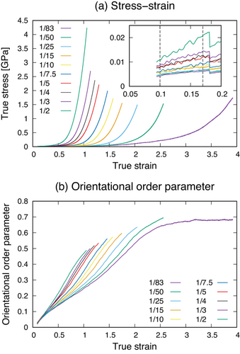
First, Figure 4 shows the stress–strain curves of iPP structures with different crosslink densities and the profiles of the orientational order parameter. Our calculations do not consider the breaking of chemical bonds, and thus the fracture of the iPP structures does not occur during the mechanical tests. To determine the fracture point, we monitored the maximum force exerted on bonds between iPP beads at each step. According to a theoretical work using a DFT method, a force of around 6 nN is required to break a C−C bond in alkanes such as ethane and butane.^[43] We defined a strain at which the maximum bond force reaches 6 nN as a fracture strain. In the stress–strain curves in Figure 4a, all of the iPP structures yield at a strain just less than 0.2 with the slight relaxation of the stress. Then, the stress increases as the orientational order parameter rises, that is, as the iPP chains become more aligned to the deformation direction. These features are in a good agreement with those observed in real materials during mechanical tests.

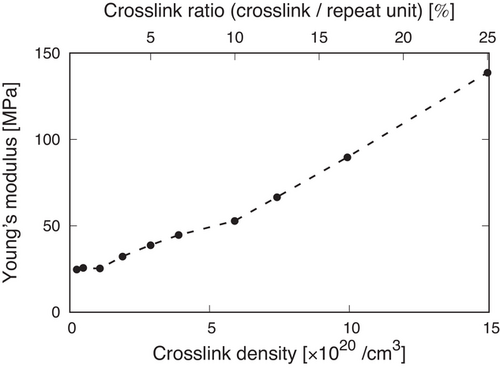
Next, to understand the contribution of crosslink density to mechanical properties, the Young's moduli of the iPP structures were evaluated from the stress–strain curves. We obtained a best-fit line for data at true strains between 0.1 and 0.17, where the stress linearly increases against true strain (see Figure 4a), and the Young's modulus was calculated as its slope. Figure 5 shows the Young's modulus as functions of the crosslink density and crosslink ratio. The crosslink ratio is the ratio between the number of crosslinks and that of the repeat unit on average. This figure demonstrates that the Young's modulus maintains an almost constant value at a crosslink density less than around 1 × 10²⁰ cm⁻³, corresponding to one crosslink every 25 iPP beads (= 50 repeat units), and then starts to increase with a rise in the crosslink density. Therefore, there is a threshold of the crosslink density above which the introduction of the crosslinks works to improve the Young's modulus. This is because the contribution of the crosslinks is limited in the region where the Young's modulus was determined due to the small strains. Experimental works reported that the introduction of crosslinks increases the Young's modulus, which is consistent with the tendency in our calculations.^[44]

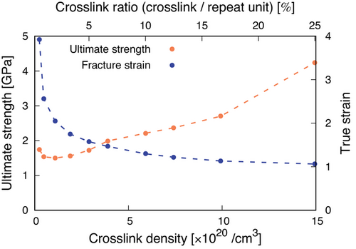
Next, we evaluated the ultimate strength and fracture strain (Figure 6). We set the stress value at a fracture strain defined above as an ultimate strength. As with for the Young's modulus in Figure 5, the ultimate strength increases with an increase in the crosslink density for values greater than around 1× 10²⁰ cm⁻³. This is in a good agreement with experimental works demonstrating that a higher crosslink density leads to a higher tensile strength in brittle polymers such as polystyrene.^[45] Additionally, the fracture strain decreases as the crosslink density increases. This indicates that iPP with a higher crosslink density breaks at a lower strain and becomes more brittle. This is also the same trend as observed in real materials including crosslinked polymers and rubbers.^[46]

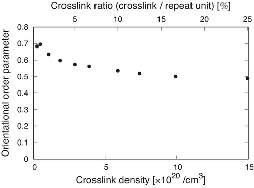
In addition to the mechanical properties such as Young's modulus and ultimate strength, some studies have reported that crosslinks also change the topology of polymers during mechanical tests.^[47] An increase in the crosslink density restricts chain alignment that can lead to strain-induced crystallization, which also significantly affects the mechanical properties. We then investigated the contribution of crosslink density to chain alignments. Figure 7 plots the orientational order parameter at a fracture strain as functions of the crosslink density and crosslink ratio. The orientational order parameter at the fracture strain was evaluated in Figure 4b. This figure shows the tendency that iPP chains with a larger number of crosslinks are less likely to be oriented along the deformation directions, which is consistent with experimental works.^[47] Thus, our calculations successfully revealed the contribution of crosslinks not only to the mechanical properties such as Young's modulus and ultimate strength but also the morphological changes during mechanical tests.

In our calculations, iPP structures are amorphous and thus do not contain crystalline phases, which differs from real iPP materials with a mixture of amorphous and crystalline phases and can affect the stress–strain behavior. Nevertheless, an experimental work suggests that, in mechanical tests at room temperature, structural changes in amorphous phases of iPP are more significant than those in crystalline phases and thus play an important role in carrying mechanical loads.^[22] As mentioned above, our calculations successfully reproduce the stress-induced alignment of iPP chains and show the tendency that this morphological change is restricted as the crosslink density increases, which is in good agreement with experimental works. Therefore, even in real materials that can contain crystalline phases, our calculations will still be helpful to understand the effect of crosslink density on the stress–strain behaviors.

Furthermore, we determined the fracture point of iPP when the maximum force reached 6 nN instead of implementing bond breaking in DPD simulations for the computational efficiency. Nevertheless, the trend of fracture strain in our calculations is consistent with that obtained by a computational work that simulated stress–strain curves of a thermoset plastic in MD simulations where bond breaking can occur during mechanical tests.^[15] Thus, the determination of the fracture points by a single bond breaking event does not significantly affect the trend in mechanical properties.

5 Conclusion

We have developed a coarse-graining procedure for iPP using Bayesian optimization and DPD. During Bayesian optimization of DPD parameters, two different cutoff distances were employed to avoid inappropriate solutions and to enhance the probability of reaching a physically meaningful optimization. Additionally, a 4–2 LJ potential was used instead of the conventional 12–6 LJ potential to reproduce the soft interactions between iPP beads. These modifications successfully worked to derive the DPD parameters that reproduce the structural properties and stress–strain behaviors compared to an all-atom MD system. This enables us to address larger iPP molecules, in which we can reproduce experimentally observed M_c values.

Applying the coarse-grained iPP with the optimal DPD parameters, we investigated the contribution of crosslink density to the mechanical properties of iPP structures with realistic crosslink densities, which assumes the introduction of physical or chemical crosslinks into recycled iPP to improve its degraded mechanical properties. Our calculations revealed that the mechanical properties such as the Young's modulus and ultimate strength increase while iPP gets more brittle with an increase in the crosslink density. This is in a good agreement with experimental observations. Our results also showed that there is a critical crosslink density above which the mechanical properties start to be improved by the further introduction of crosslinks.

In real materials including iPP, mechanical properties can be affected by many parameters such as crystallinity and molecular weight in addition to crosslink density. Our calculations reveal the pure contribution of crosslink density to mechanical properties and topological changes during mechanical tests. This can help us to relate the trend of mechanical properties observed in experiments to crosslink density and to achieve targeted properties by the introduction of physical or/and chemical crosslinks.

Conflict of Interest

The authors declare no conflict of interest.