
A novel similar habitat potential model based on sliding-window technique for vegetation restoration potential mapping
Abstract
Vegetation restoration potential mapping (VRPM) is of great importance for regional ecosystem restoration planning after long-term land degradation or short-term disasters. However, there are some problems to be solved in the current models for evaluating the potential of vegetation restoration. First, the models for VRPM are mostly established based on a knowledge-driven index system. Although this kind of model is logically rigorous, it relies too much on expert knowledge and is relatively inefficient, especially for large-area vegetation restoration assessments. Second, because of the spatial heterogeneity, as well as the absence of important indicators, the traditional global-based evaluation models are difficult to adapt to the entire study area. In this study, an improved data-driven approach, that is, a sliding-window based similar habitat potential model, is developed for VRPM. The advantages of the new model include: (a) it is more efficient in determining the importance of each influencing factor without resorting to expert knowledge; (b) it is more locally adaptive than the global model because it performs sample training, rule building, and vegetation restoration potential calculation in each current local window. We provide a case-study to show the modeling process and result interpretation of the new model.
1 INTRODUCTION
Land degradation refers to the process of land suffering because of the interference or destruction caused by human factors (Kéfi et al., 2007; Zhang et al., 2014; Bajocco et al., 2018), natural factors (Bednář & Šarapatka, 2018), or the combination of both human and natural factors (Hammad & Tumeizi, 2012; Salvati et al., 2014; Stringer & Harris, 2014). As a result, the environment degenerates, and the original productivity of the land gradually declines (Lal, 1993; Zhang et al., 2007; An et al., 2008). Thus, an important prerequisite before making a plan for restoring local terrestrial ecosystems is to evaluate the potential of the vegetation in the degraded land, and a vegetation restoration potential map can help to improve the efficiency of ecosystem restoration (Broncano et al., 2005; Bisson et al., 2008; Gutierres, 2014).
Previous studies on vegetation restoration potential mapping (VRPM) are mainly focused on vegetation restoration and reconstruction after natural disasters such as forest fires (Cerdà & Doerr, 2005; Ireland & Petropoulos, 2015), earthquake disasters (Prabakaran & Paramasivam, 2014; Liu et al. 2017b), floods (Harwell & Havens, 2003, Meitzen et al., 2018), and mining activities (Allred et al., 2015; Nauman et al., 2017). Other studies have evaluated the suitability of vegetation or species for ecological restoration from the perspective of natural potential vegetation (Westhoff & van der Maarel, 1978; Franklin, 2010). However, there is very limited research concerning the evaluation of regional vegetation restoration potential for land degraded by human activities (Cantarello et al., 2011). China has made great efforts and significant achievement in vegetation restoration in ecologically fragile areas (Yin, 2009; Bryan et al., 2018), which has led Chinese scholars to paying more attention to VRPM (e.g., Jiao et al., 2005; Liu et al., 2017a; Zhao et al., 2017).
In practice, multifactor comprehensive evaluation (MFCE) models are generally applicable for VRPM (Broncano et al., 2005; Bisson et al., 2008). The conceptual basis of MFCE models is to select suitable indicators according to the overall goals to be achieved, to group and combine the indicators in a hierarchical manner according to their inter-relevance and affiliation, and ultimately to convert the multiple indicators into a single indicator that can comprehensively reflect the score of the object to be evaluated (Bisson et al., 2008). The steps for the application of MFCE models in VRPM are the following: (a) select appropriate factors which contain several subfactors that can affect vegetation growth, (b) determine the weights of the factors and subfactors, (c) calculate the score for each object on each factor and subfactor, and (d) integrate the scores of all factors and obtain a comprehensive index for each object. The key of the application of MFCE in VRPM is thus to build an indicator system and determine the weight for each indicator. With regards to the construction of an indicator system, Bisson et al. (2008) selected soil type, vegetation cover, slope elevation, topography, and geology; Yan et al. (2014) designed a hierarchical index system including site conditions and ecological memory to evaluate the resilience of forest ecosystems, where the former includes terrain, soil, climate, water, and human disturbance, and the latter includes both internal and external memories; Dong et al. (2015) constructed an evaluation index system for the restoration potential of river basin ecosystems from three aspects, that is, site condition indicators, vegetation status indicators, and climate indicators. Related research also includes natural potential vegetation mapping, where solar radiation, topographical condition, wind exposition, soil, and geology are the most commonly used environmental variables for species distribution modeling (Gutierres, 2014; Gutierres et al., 2015, 2018). In terms of methods to determine index weights, Chen and Li (2008) first used the scale ratio table to score the influencing factors, and then they used an improved analytical hierarchy process (AHP) method to determine the weight of each indicator; Arianoutsou et al. (2011) used the ratio estimation method for weight determination on the basis of a decision matrix; Yan et al. (2014) used the AHP and the coefficient of variation methods to determine the index weights; and Li et al. (2015) constructed the judgment matrixes for the target layer, the criterion layer, and the indicator layer through determination of weights via expert ranking.
In MFCE models, index weights are mainly determined based on expert knowledge, that is, the determination of weight depends on the judgment of experts. The acquisition of expert knowledge requires a process of field exploration and indoor summarization. In a relatively small area, knowledge is relatively easy to establish; however, for regional scale research, this practice appears to be less efficient (Gallet & Sawtschuk, 2014; Peng et al., 2019). With the development of remote sensing technology, more and more vegetation coverage data set products become available, which makes it possible to study vegetation coverage change and its responses to environmental variables at regional and even larger scales (Tang et al., 2012; Fernandez-Manso et al., 2016; Li et al., 2020). Because the vegetation index is a direct reflection of the state of vegetation growth, the maximum potential for vegetation restoration can be obtained by studying the optimal growth state of vegetation in different habitats (Gao et al., 2017; Nauman et al., 2017). Therefore, in recent years, some scholars have begun to study the vegetation restoration potential at the regional scale based on data-driven methods supported by remote sensing data (e.g., Gao et al., 2017; Nauman et al., 2017; Peng et al., 2019). For instance, Gao et al. (2017) divided its study area into similar habitat units according to soil conditions, topographic conditions, and meteorological conditions using statistical methods and geospatial analysis techniques. Subsequently, according to the rule that similar habitats lead to similar landscapes, the vegetation potential of the Loess Plateau was evaluated by using Systèm Pour l'Observation de la Terre-VEGETATION (SPOTVEG) normalized difference vegetation index (NDVI) data. Gao et al.'s (2017) model is established based on the outcomes of vegetation growth rather than the expert's judgment and thus can improve the efficiency of VRPM. However, it still belongs to a global model and suffered from following disadvantages. First, the model established at the whole study area is difficult to fit each location. The larger the scope of the study area, the worse the applicability of the global model, which is determined by the spatial differentiation law in Geography (Rutchey & Godin, 2009; Siles et al., 2010). Second, due to the limitations of human cognition and the difficulty of data acquisition, some potential environmental variables may be difficult to obtain or measure (Strohbach, 2018; Zhang et al., 2018b). As a result, missing variables are inevitable in scientific research, which will affect the similar habitat division, and thus increase the risk of bias in the evaluation results.
- The vegetation restoration potential index (VRPI) is calculated at each current location based on the same natural conditions within its local window. This makes the SWSHPM model be able to allow environmental variables to have different effects on vegetation growth at different locations, so as to overcome the spatial heterogeneity of environmental variables and improve the accuracy of evaluation results.
- According to Tobler (1970), nearby things tend to show closer relationship than distant things in space; the theory of regionalization suggests that variables with longer ranges show slower spatial changes (Goovaerts, 1997, p. 38). It can be imagined that missing environmental variables that change over macroscales with relatively long range are tend to be stable within a certain range (Koutsias et al., 2010; Zhang et al., 2018b), and thus its effects on vegetation growth may be very limited when establishing a VRPM model at a local window scale. Hence, the SWSHPM model is expected to weaken the risk caused by missing important variable(s) in a global VRPM model.
The rest of this paper is organized as follows. In the next section, we outline our new developed model—the SWSHPM model, before which traditional similar habitat vegetation restoration potential model is described firstly as fundament. In Section 3, a case-study is provided to demonstrate the application of the SWSHPM. In Section 4, detailed explanations and analyses are given to the study case. In Section 5, we discuss the characteristics of the new model and the reliability of its application. Finally, some conclusions and closing remarks are made in Section 6.
2 MODEL DESCRIPTION
2.1 Similar habitat vegetation restoration potential model
Generally, areas with similar natural conditions have similar landscape and vegetation coverage (Gao et al., 2017; Nauman et al., 2017). For instance, the natural landscape and vegetation coverage should be similar under the same terrain conditions (e.g., elevation, slope, and aspect), climatic conditions (e.g., precipitation, temperature, and humidity), and soil and geological conditions (e.g., pH level, soil thickness, element content, and formation). If vegetation coverage differences exist in the range that owns the same natural conditions, it means that there is potential. Therefore, the difference between the vegetation index (VI) of each location and the maximum VI under that habitat can be calculated to measure the potential vegetation growth at that location (Gao et al., 2017).
 (1)
(1)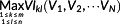 means to find the maximum VI from the cells which take the same values as the current cell in the variables of V1,V2,⋯VN and then take this maximum value as the return value. Supposing that there are m rows and n columns in the whole study area, VIij(V1, V2, ⋯VN) is the VI value taken by the current cell.
2.2 SWSHPM model
 (2)
(2)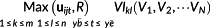 means to find the maximum VI from the cells belong to different years' VI map (y ¯ b means the beginning year and y¯ e means the end year), which take the same values as the current location in the variables of V1,V2,⋯VN and then take this maximum value as the return value. Suppose that there are m rows and n columns in the local window, VIij(V1, V2, ⋯VN) is the VI value taken by the current cell for a giving year.
As in other local window models, one problem with the SWSHPM model is the determination of the local window size R. In geographically weighted regression (GWR) model, one can determine the window size either using a quantitative method like Akagi information (Hurvich et al., 1998) or just experience (Su et al., 2012). In this study, we chose the latter.
3 CASE-STUDY
In order to further describe the SWSHPM model and demonstrate the modeling process used in VRPM, Shaanxi Province of China is taken as an example in this study.
3.1 Study area
Located in central China, Shaanxi province is divided into three parts according to different natural geography and human environment, that is, northern Shaanxi, Guanzhong, and southern Shaanxi (Figure 1). Located in the Loess Plateau, northern Shaanxi has two municipalities, Yan'an and Yulin. It is mainly dominated by hilly and gully landforms, although it is relatively flat near the adjacent Inner Mongolian Plateau. Guanzhong is located along the Weihe River, including the four municipalities of Xi'an, Xianyang, Tongchuan, and Baoji, which are mainly distributed in the low-lying Guanzhong Plain. The rest part of Shaanxi located to the south of the Qinling Mountains is called southern Shaanxi, which belongs to the Qinba mountain area, including the three municipalities of Shangluo, Ankang, and Hanzhong. During the 1970s to 1990s, with mounting pressures of population growth and economic development, the ecological environment in western China continued to deteriorate, and land degradation was severe (Yang et al., 2005). In order to suppress and reverse the ecological degradation, the Chinese Government introduced a series of ecological policies and implemented a series of ecological projects, including the construction of the Three-North Shelterbelt, the Ecological Cultivated Land Conversion Project, and the Natural Forest Protection Project (Wang et al., 2010; Yin & Yin, 2010; Qiu et al., 2017). After nearly 20 years of efforts, the vegetation coverage in Shaanxi has been greatly improved (Cao et al., 2009; Liu et al., 2010).

3.2 Data sources and preprocessing
VI data are used here to indicate vegetation coverage. Regarding natural condition variables, previous studies have mostly considered the effects of meteorology, soil, geology, and topography on vegetation restoration (e.g., Laughlin, 2014; Li et al., 2015). In this study, vegetation restoration potential is calculated based on the SWSHPM model. At a region scale, the regional climate conditions are very similar, and their effect on the vegetation growth can be neglected (Bisson et al., 2008; Nauman et al., 2017), and the influence of geological environment can be reflected greatly by soil type data (Krasilnikov et al., 2011; Zeraatpisheh et al., 2017). In a relatively limited range of the local window used for VRPM in this study, the regional climate condition changes are even smaller. However, topoclimate conditions are important factors for the division of similar habitat units and should be included in the model. Thus, terrain conditions including the elevation, ground slope, and aspects, which are the composition elements for the formation of topoclimate, are put in the model. Besides, soil type is also taken into account because it can reflect the environment differences for vegetation growth at local window scale. Therefore, these natural condition variables are used to build similar habitats for VRPM here. All variables used in this study are expressed in the form of geographic information system (GIS) raster data using the World Geodetic System 1984 (WGS-84) projected coordinate system, with 111°E as the central meridian and Universal Transverse Mercator (UTM) as the projection.
The maximum synthetization of the VI values from 2000 to 2016 is used to calculate the maximum potential for vegetation restoration, and then the difference between the VI in 2000 and the corresponding maximum potential value is calculated as the LVRPI. Besides, the growth rate of the VI from 2000 to 2016 is calculated to verify the validity of the LVRPI, because the greater LVRPI should result in greater growth rate of the VI generally.
3.2.1 Topographic and soil data
The topographic data used in this study was downloaded in Advanced Spaceborne Thermal Emission and Reflection Radiometer (ASTER) Global Digital Elevation Model (GDEM) format from the geospatial data cloud platform of the Chinese Academy of Sciences (http://www.gscloud.cn) with a spatial resolution of 90 m × 90 m. The downloaded original data were masked to the study area to obtain the elevation raster layer (Figure 1). By using the surface analysis tools in ArcToolbox in ArcGIS10.2, layers of terrain slope and aspect were obtained, as shown in Figure 2a,b, respectively.

The vector soil type map at the scale of 1:1,000,000 of the study area was derived from the Institute of Soil Science, Chinese Academy of Sciences (Shi et al., 2004, 2006), which was converted to raster dataset with a spatial resolution of 90 m × 90 m. The new rasterized layer for soil type was further masked to the study area to obtain the soil type raster layer, as shown in Figure 2c.
3.2.2 Vegetation index data
VI is an empirical measure of vegetation growth state by means of remote sensing. The Moderate Resolution Imaging Spectroradiometer (MODIS) provides a variety of spatial and temporal resolution vegetation index products. In this study, the MOD13Q1 data set (Version 6; Didan, 2015) of the synthetic vegetation index product with the highest spatial resolution (250 m × 250 m) and a time resolution of 16 days was selected. The version of this data was published in 2015, and two vegetation index products were provided, that is, the NDVI and the enhanced vegetation index (EVI); other kinds of VIs, such as soil-adjusted vegetation index and topographic wetness index (Hunt et al., 2013; Leitão & Santos, 2019), can be obtained through band operation to the original multispectral bands. According to Li et al. (2010) and Gu et al. (2013), EVI could better distinguish the vegetation coverage differences than other VI products in high vegetation coverage area. There are various types of land use in the study area, including both low vegetation coverage areas, such as cultivated land, waters, construction land, and unused land, and high vegetation coverage areas, such as forest land and grassland. During the process of ecological engineering implementation, vegetation restoration is caused not only by the conversion of the original sloping cultivated land to forest land and grassland which can be well reflected by all kinds of VIs mentioned above, but also by the further vegetation coverage improvement of the original forest land and grassland which only can be better measured by EVI. As a result, EVI was thus adopted in this study. The average of the EVIs obtained during the vegetation growth period, that is, the 97th day to the 289th day, was used as the annual EVI.
The study area falls completely within the two MODIS scenes of H26V05 and H27V05. In order to keep the same range and cell resolution with the topographic data, mosaic was performed for the two EVI scenes with the study area range as a mask, and the resample cell size was 90 m × 90 m raster data. Figure 3a,b is the obtained EVI layers for the study area in 2000 and 2016, respectively. The EVI maximum synthesized layer from 2000 to 2016 was obtained in Figure 3c.

4 RESULTS AND ANALYSES
4.1 Construction of similar habitat
Classification layers were used to construct similar habitats. The classification layers were derived from the discretization of the natural condition variables that have potential impacts on the vegetation growth, that is, the V1,V2,⋯VN in Equation 2. As mentioned in Section 3, the elevation, ground slope, aspects, and soil type were used as the classification layers for the construction of similar habitats in this study. Because vegetation restoration is usually considered only in the area where the slope is above 15° in China's Sloping Land Conversion Program [Grain for Green (GFG); Liu & Lan, 2015] and it is almost impossible to perform GFG in area less than 6°, the area below 6° in this study was masked from the study area. As a result, the terrain slope map was finally divided into a four-class layer, that is, 6–15° (V1 = 1), 15–20° (V1 = 2), 20–25° (V1 = 3), and 25° and above (V1 = 4); the variable of the slope aspect was divided into an eight-category layer, that is, the east (V2 = 1), the southeast (V2 = 2), the south (V2 = 3), the southwest (V2 = 4), the west (V2 = 5), the northwest (V2 = 6), the north (V2 = 7), and the northeast (V2 = 8); there are 72 types of soils involved in the study area, which means that the soil type variable takes 72 distinct values; in addition, we classified the elevations by equal interval method, and the study area was divided into 180 types of elevation intervals. Through the combination of these four layers, 4 × 8 × 72 × 180 = 414,720 similar habitats can be formed at most theoretically in the whole study area, as shown in Table 1.
| ID | Slope grade (V1) | Aspect category (V2) | Soil type (V3) | Elevation classes (V4) | Category code |
|---|---|---|---|---|---|
| 1 | Aa | Bb | Cc | Dd | A × 106 + B × 105 + C × 103 + D |
- a A takes the values of 1, 2, 3, and 4.
- b B takes the values of 1, 2, … , 8.
- c C takes the values of 1, 2, … , 72.
- d D takes the values of 1, 2, … , 180.
According to the similar habitat classification value at the current position, for example, i = 2,716, j = 3,648, and the classification value is 2,413,162, a similar habitat set can be obtained from the current local window with the size of R = 21 × 21 cells. As shown in Figure 4a, the current position is in boldface, and the cells belonging to the same similar habitat unit as the current location are highlighted in yellow background.

4.2 Mapping of LVRPI
The window slices corresponding to the position of Figure 4a are extracted from Figure 3a,c, respectively, as shown in Figure 4b,c. It can be seen that the maximum synthesized EVI from 2000 to 2016 in this similar habitat is 0.22, which is in boldface highlighted in red in Figure 4c, while the current position EVI in 2000 is 0.14, which is in boldface in Figure 4b. Therefore, the LVRPI calculated for the current position (i = 2,716, j = 3,648) is 0.08 according to Equation 2.
Figure 4 only shows a general process for the calculation of the LVRPI with a simple sample set. In practice, more details should be considered. First, the size of the window needs to ensure that there are enough samples in the window (Xiao et al., 2016), and that the values of the possible missing variables in the window are sufficiently similar so that they can be ignored (Koutsias et al., 2010; Zhang et al., 2018b). The local window size was finally determined as 201 cells × 201 cells, that is, 18 km × 18 km. Second, in order to avoid uncertainty of the data, the 0.98 fraction of the maximum distribution of the EVI was used instead of the maximum value in calculating the LVRPI. Using the Excel VBA, a software module for the LVRPI, that is, SWSHPM model was developed. By using both the SWSHPM model and the related tools provided by the ArcToolbox in ArcGIS 10.2, the map of LVRPI was finally obtained in Figure 5a.

4.3 The spatial distribution for vegetation restoration potential
As can be seen from Figure 5a, there is a large spatial difference in vegetation restoration potential in the study area in 2000, and the spatial change of the LVRPI shows a definite trend and regularity. High LVRPI values are more concentrated in Yan'an of northern Shaanxi and Shangluo in southern Shaanxi; while low LVRPI values are more likely to appear in Hanzhong and Ankang in southern Shaanxi, Xi'an in Guanzhong, and Yulin in northern Shaanxi. In Baoji of Guanzhong, there is a greater vegetation restoration potential in the northwest, while the vegetation restoration potential in the remaining areas is relatively small.
Generally, higher LVRPI indicates that the vegetation is easier to recover, but it also means that the land degradation caused by human activities was more serious. Lower LVRPI means that there is relatively smaller human disturbance, and the vegetation has been relatively fully regrown under the current resource endowment conditions; therefore, it also indicates that there is relatively less potential for further increase of vegetation coverage.
- First, there is a large concentration of high LVRPIs in Yan'an of northern Shaanxi, indicating that its land degradation was more serious at the end of the last century, which is why the Chinese Government chose Yan'an as a pilot for the GFG Program at that time (Yin & Yin, 2010).
- Second, Yulin, located in the farming-grazing transitional zone between the Loess Plateau and the Inner Mongolia Plateau, shows relatively lower LVRPI values in its administrative counties. One possible reason is that the increase of latitude coupled with the continental climate causes the precipitation and temperature conditions to deteriorate, such that the land cover is more characteristic of herbaceous plants (Zhang et al., 2006). Due to the shorter growth cycle of grasses, the maximum potential for vegetation growth is reduced. As a result, the LVRPI level there is generally low.
- Finally, in Guanzhong and southern Shaanxi, the high LVRPI values are mainly concentrated near the boundary between Shaanxi and its neighboring provinces. These locations used to be rich in forest resources, and thus the high LVRPI values there suggest a large amount of forest degradation caused by over-logging (Zhang et al., 2019b). China's Natural Forest Protection Project, which restricts logging activities and protects remaining natural forests in many parts of the country including Shaanxi, was launched in year 2000 (Xu et al., 2018). Prior to that time, illegal logging was prevalent in places under weak governance, such as the border areas between neighboring provinces.
5 DISCUSSION
5.1 SWSHPM's advantage in dealing with spatial heterogeneity
Heterogeneity is an important problem in statistical modeling, which usually happens when samples are from different populations (Becker et al., 2013). It can be avoided more or less by modeling the samples separately according to their population, for example, subgroup regression (Karali et al., 2013). In spatial statistics, heterogeneity usually manifests as spatial heterogeneity. For instance, in the presence of spatial heterogeneity, the distribution of residuals will show spatial trends or dependencies if a global regression model is established (Breitenecker & Harms, 2010; Perez-Verdin et al., 2014). In some research of vegetation restoration, scholars also pay attention to spatial heterogeneity. For instance, Zhang et al. (2018a) found that the contribution of policy to vegetation restoration is different at different locations in the study area; in different locations, the increase in vegetation coverage due to unit input is also different. Besides, it is found that the importance of water to the growth of vegetation is also different among different areas (Jing et al., 2011; Zhang et al., 2017).
With respect to the potential of vegetation restoration, it is generally considered to be determined by terrain conditions, climatic conditions, and soil and geological conditions (Bisson et al., 2008; Gutierres, 2014; Nauman et al., 2017). However, due to the existence of spatial heterogeneity, the contribution of these factors to vegetation growth may change with the change of position, which means that the potential for vegetation growth will be no longer the same in the same similar habitat unit.
In this study, we developed the SWSHPM model to establish a vegetation restoration potential measurement model in each local window. Because the samples within a local window are more similar and more closely related (Fotheringham et al., 1996), it is more likely to come from the same population (Gaucherel, 2007). Therefore, the new model can overcome or at least weaken the adverse effects of spatial heterogeneity, thereby improving the accuracy of vegetation restoration potential measurement.
5.2 SWSHPM's advantage in dealing with missing variables
Missing variables is another important problem in statistics (Clarke, 2005, 2009). Although statistic models should be established based on the assumption that there are no important unknown variables, and a series of statistic such as R2 can be used to test the explanatory power of the model, it is difficult to ensure that the selected independent variables have sufficient explanatory power for the target variable in reality (Clarke, 2005). Sometimes, in order to solve the actual problems, regression analysis can be performed even if the R2 value is quite small (Ramsey, 1969). However, it is an indisputable fact that in spatial statistics, the use of the GWR model can greatly increase the value of R2, although the independent variables used in GWR are identical to the classical global regression (Szymanowski & Kryza 2011; Zhang et al., 2018a). Why could R2 be increased without increasing the number of independent variables when GWR is used instead of global regression? We believe the answer is that those variables that are missing or not included in the model may have certain spatial trends and autocorrelation; although they vary widely throughout the study area, the changes in a partial window are relatively small (Koutsias et al., 2010; Zhang et al., 2018b).
The sliding-window algorithm is applied in this study for VRPM, which is also for the purpose of eliminating or weakening the influence of missing variables. Because the missing variables have spatial autocorrelation and trend, it can be sure that the new developed model can weaken the influence of unknown or missing variables in VRPM more or less.
5.3 The reliability of the SWSHPM model
In Section 4, we analyzed the spatial distribution for the vegetation restoration potential obtained by our model, and our results are consistent with natural and socioeconomic conditions in Shaanxi Province, as well as previous studies, proving the reliability of our model to some extent. To further evaluate the reliability of the LVRPI, we can also verify whether locations with higher potential have a faster restoration rate in general.
To that end, the growth rate for EVI from 2000 to 2016 was calculated for each cell, and the resulting layer was further aggregated to county level. Similar with Figure 5b, the descending order ranking of the annual average vegetation growth rate was obtained. Figure 6 shows the scatter plot distribution of the counties in the study area, with the LVRPI based on EVI as the abscissa and the annual growth rate for EVI as the ordinate. The result shows that in the areas with high potential, the vegetation restoration rate is also high, and the R2 is as high as 0.6304, which means that the 63.04% of the vegetation restoration can be explained by LVRPI.

With respect to the other 37%, it should be explained by the ecological restoration policies and the effectiveness of the implementation. For instance, Wuqi County was ranked as 59 in terms of the LVRPI, but the rank of its annual growth rate was 34 in the study area. This is mainly due to the unusually strong implementation of the Sloping Land Conversion Program, as well as the county's more stringent protection of the afforested sites than many other counties (Zhang et al., 2018a, 2019a).
To sum up, the LVRPI proposed in this study can satisfactorily predict the potential of future vegetation restoration.
6 CONCLUSIONS
This study proposes a novel data-driven model (the SWSHPM) for VRPM. The new model is developed based on sliding-window technique and owns the following features: (a) it can effectively reduce the adverse effects that the spatial heterogeneity brings in computing the VRPM; (b) it can somewhat overcome the influence of missing variables on evaluating vegetation restoration potential; and (c) it can efficiently calculate and obtain relatively accurate vegetation restoration potential across the whole province. The case study demonstrates that the LVRPI mapping obtained by the SWSHPM model is reliable and thus can provide decision-making reference for vegetation restoration planning.
At a time when the international community is aiming to restore 350 million ha of deforested and degraded land by 2030 (International Union of Conservation Networks (IUCN), 2012), there has emerged a great need to develop more practical and effective restoration planning and monitoring tools. Given that ecological restoration is often an undertaking combining biological and engineering measures, we feel that the model we have built for evaluating the vegetation restoration potential can be of broad relevance and interest. Although there may be some areas for improvement with the model, as a new analytical framework considering spatial heterogeneity, it is expected to be refined to evaluate the vegetation restoration potential of degraded landscape and even take into account of the potential of ecosystem service provision by moving beyond evaluating the vegetation restoration potential only.
ACKNOWLEDGMENTS
This study benefited from joint financial support by the Programs of National Natural Science Foundation of China (nos. 41602336, 71503200, and 71603209), the China Postdoctoral Science Foundation (no. 2017T100773), the Special Scientific Research Fund of Forestry Public Welfare Profession of China (no. 201504424), and the Fundamental Research from Northwest A&F University in 2017 (no. 2017RWYB08). We would also like to thank Editage (www.editage.cn) for English language editing.