Applying deep learning to quantify empty lacunae in histologic sections of osteonecrosis of the femoral head
Abstract
Osteonecrosis of the femoral head (ONFH) is a disease in which inadequate blood supply to the subchondral bone causes the death of cells in the bone marrow. Decalcified histology and assessment of the percentage of empty lacunae are used to quantify the severity of ONFH. However, the current clinical practice of manually counting cells is a tedious and inefficient process. We utilized the power of artificial intelligence by training an established deep convolutional neural network framework, Faster-RCNN, to automatically classify and quantify osteocytes (healthy and pyknotic) and empty lacunae in 135 histology images. The adjusted correlation coefficient between the trained cell classifier and the ground truth was R = 0.98. The methods detailed in this study significantly reduced the manual effort of cell counting in ONFH histological samples and can be translated to other fields of image quantification.
1 INTRODUCTION
Osteonecrosis of the femoral head (ONFH), also known as avascular necrosis, is a disease condition caused by the inadequate blood supply to the subchondral bone, resulting in the death of cells in the bone marrow.1 More than 20,000 new cases of ONFH are diagnosed every year in the United States alone.2 Decalcified histology is a commonly used method to analyze tissue specimens,3 and in histology images of femoral head tissues, the presence of empty lacunae has been widely accepted as an indicator of osteocytic cell death and ONFH.4 However, quantifying the severity of the disease condition ex vivo typically requires manual cell counting of histological specimens by researchers with significant expertise and training time. To this end, we sought an automated way to discern the percentage of empty lacunae in histology images of different treatment groups for early stage avascular necrosis, in which accuracy of algorithmic cell counting would be cross-validated with manual cell counting.
The MATLAB Image Processing Toolbox contains algorithms and tools to automate a personalized image processing workflow.5 We first developed a multi-cell counting algorithm using the MATLAB Image Processing Toolbox, in which we tuned edge detection, noise filtering, and image overlaying thresholds to distinguish osteocytes from empty lacunae. To improve counting accuracy and increase throughput, we proceeded to train a deep convolutional neural network and develop a binary classifier that automatically detects the number of osteocytes and osteocytic empty lacunae within a single image. To confirm that this approach could be applied to more complex multi-class object detection scenarios, particularly since empty lacunae percentage is only one index of early stage osteonecrosis, we further developed a multi-class model that classifies healthy osteocytes, pyknotic osteocytes, and empty lacunae. Faster-RCNN is a widely used object detection framework in face detection and computer vision spheres that utilizes deep convolutional networks for rapid image classification.6-8 Using the Faster-RCNN framework, we developed a cell classification and quantification tool that significantly increases counting accuracy and reduces manual effort and processing time. Although other researchers have used deep learning to evaluate and diagnose ONFH based on MRI images,9 to our knowledge, this study is the first application of deep learning to quantify the percentage of empty lacunae in histological images and has the potential to assist researchers and physicians in classifying and evaluating the treatment efficacy of early stage ONFH.
2 MATERIALS AND METHODS
2.1 Haemotoxylin and eosin staining and imaging
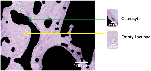
A total of 27 femoral heads in a model of steroid-associated ONFH in rabbits were used.10-12 After fixation in 4% paraformaldehyde (pH 7.4) and decalcification in 0.5 M ethylenediaminetetraacetic acid (EDTA, pH 7.4), the specimens were embedded in optimal cutting temperature (OCT) compound and cut into 8-µm-thick longitudinal sections, which were then stained with hematoxylin and eosin (H&E) before imaging. All images were taken with a digital microscope (BZ-X-710, Keyence) at 200× magnification, following a standard protocol for unbiased representative sampling. Before processing the images further, the surrounding bone marrow regions were removed (blacked out) using ImageJ to eliminate potential artifacts (Figure 1). A total of N = 135 images were used in this study.
2.2 Manual counting
As an initial verification step, a random subset of the full sample size of images was selected for manual counting (N = 27). For each selected image, the osteocytes and empty lacunae were counted manually using ImageJ (Figure S2). Within the ImageJ interface, osteocytes and empty lacunae were marked by clicking the cells, and the counts for each were tallied separately. The manual counting procedure was repeated twice by two independent researchers with experience in ONFH histological studies, and all data collection results were blinded until counting was complete. After the initial verification, the full set of images (N = 135) was manually counted. All images were manually counted independently of software analysis and development in both stages. For the labeling of three classes, osteocytes (healthy), pyknotic cells, and empty lacunae, a systematic decision tree comprising three independent evaluators was used to establish the ground truth (Figure S3).
2.3 Developing an automated multi-cell counting algorithm in MATLAB
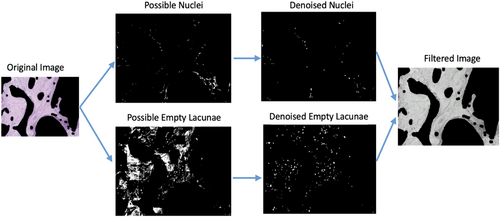
Histology images were first separated into hue (H), saturation (S), and value (V) channels in MATLAB. The H, S, and V threshold boundary values for osteocytes and empty lacunae were then defined by manual selection using the data cursor in the MATLAB Figure toolbar. Next, the potential osteocytes and empty lacunae were identified using the edge detection feature in the MATLAB Image Processing toolbox. Holes, or closed circular features that likely indicate cells, were filled in. A series of background denoising algorithms were then applied via Gaussian filtering to remove unconnected patterns and closed features smaller than the minimum size threshold of a single nuclei (Figure 2). Finally, the identified nuclei and empty lacunae features were circled in blue and green, respectively, and overlaid on a grayscale version of the original image (Figure 3). The number of circled features (osteocytes and empty lacunae) were exported to an external spreadsheet for each treatment group, where the percentage of empty lacunae was analyzed.

2.4 Training the convolutional neural network
2.4.1 Image preprocessing
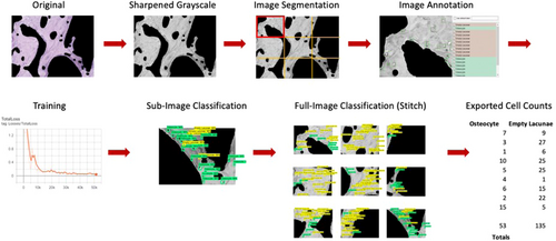
All full-sized histology images (N = 135) were converted to grayscale in MATLAB to reduce the number of color channels during neural network training. Each full-sized image (1920 × 1440 pixels) was segmented into nine sub-image blocks (1030 × 741 pixels), and each sub-image (n = 1215) was sharpened using the imsharpen tool in the MATLAB Image Processing Toolbox5 to enhance the features of interest and reduce training convergence time. Note that N denotes a full-sized image and n denotes a sub-image (1/9) in size (Figure 4).
2.4.2 Preparing the training and validation set
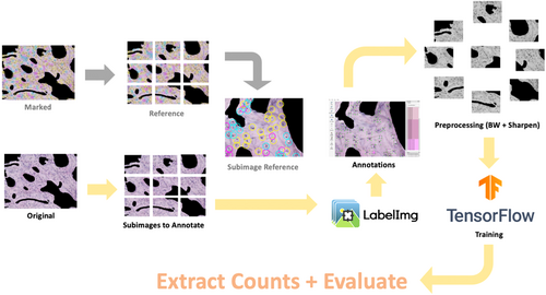
The same random subset of images (N = 27) used in the initial manual counting verification was used to train the convolutional neural network. After segmenting the images into sub-images (n = 243), a subset of the sub-images (n = 135) was randomly selected for training and validation. The training set (n = 108) and validation set (n = 27) were prepared according to the Pareto principle, also known as the 80/20 rule.13, 14 LabelImg was used to annotate each sub-image within the training and validation sets. In each sub-image, osteocytes and empty lacunae were manually annotated (boxed), and their respective coordinate locations within the image were saved in an.xml file. For the multi-class model, images were segmented and divided into training and validation sets following the same procedure. Each sub-image was then labeled using three classes—osteocytes (healthy), pyknotic cells (malformed osteocytes with peripherally displaced nuclei), and empty lacunae. Reference images with ground truth labels were used to annotate all sub-images (Figure 5).
2.4.3 Training using Faster-RCNN
Tensorflow (v.1.15) and the Tensorflow Object Detection API15 with the Inception ResNet V2 feature extractor (l = 164 layers) were used to train the neural network architecture, downloaded directly from the Tensorflow Object Detection GitHub repository.16 The.xml files from the annotated sub-images were used to create.csv files containing the coordinate positions of all features defined in the training and validation images. After generating the test labels, a new label map was created to define the classes, wherein “Osteocyte” was assigned an ID number of 1, and “Empty Lacunae” was assigned an ID number of 2. Next, record files (storing data as a sequence of binary strings) for training and validation were generated. The object detection training pipeline was configured to have two classes (osteocyte and empty lacunae) for the binary classifier and three classes (osteocyte, pyknotic, and empty lacunae) for the multi-class model, and the appropriate input and output paths for the training and testing files were defined. Default settings for the learning rate (α = 0.002), regularization hyperparameters, batch sizes, and epochs were used. To begin training, the train.py file16 was executed in Terminal with the appropriate pipeline configuration path and directories defined. Training continued until the reported loss value, a cumulative measure of the error between the predicted and observed outputs,17 consistently fell below 0.05.
2.4.4 Extracting cell counts
After training was user terminated, a frozen inference graph (.pb) was generated that contained the trained cell classifier. A separate Python script, a modification of Object_detection_image.py18 was run (Python IDLE) to extract the osteocyte, empty lacunae, and pyknotic cell counts of all the sub-images within a directory and write the data for each treatment group to a separate external spreadsheet. The total osteocyte, empty lacunae, and pyknotic cell counts were then summed automatically for all sub-images to obtain the total cell counts for each sample.
3 RESULTS
3.1 Manual counting validation
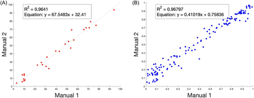
As data from manual counting was used as the ground truth for evaluating the accuracy and efficacy of the trained cell classifier, confirming the internal consistency in our manual count data was an important first step. We found a high correlation (R = 0.98, Figure 6) between the manual counts of both the initial verification step with a random subset of images (N = 27, Figure 6A) and with the full set of images (N = 135, Figure 6B).
3.2 Algorithmic multi-cell counting versus manual counting
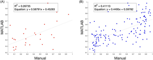
By initial visual inspection, the MATLAB multi-cell algorithm seemed to passably distinguish osteocytes from empty lacunae with noticeable small-scale noise (Figure 3). However, in comparing the quantified data from the MATLAB multi-cell counting algorithm with data from manual counting, the discrepancy between the two methods was significant for both the random subset (Figure 7A, R = 0.52, N = 27) and the full data set (Figure 7B, R = 0.64, N = 135). Although small improvements in the algorithm accuracy were achievable by further segmenting individual images, tuning the threshold values, and implementing additional image preprocessing steps (Gaussian filtering, Richardson–Lucy deconvolution, and image sharpening), the improvement to user input effort ratio was low. After further analysis, we concluded that our multi-cell counting algorithm lacked robustness when processing histology images with blurry features or low color contrast, both of which are random artifacts of the H&E staining and imaging process. Furthermore, tuning individual image threshold parameters for these cases required ample time and expertise, which defeated the purpose of our initial aim to develop an automated cell-counting platform. To overcome this problem, we decided to develop an automatic cell classifying and counting system by implementing and training an established convolutional neural network framework.
3.3 Faster-RCNN cell classification versus manual counting
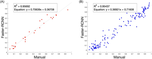
Using the independently obtained manual count data as the ground truth, we evaluated the accuracy of the cell classifier obtained from Faster-RCNN training. After analyzing a directory containing preprocessed images from the entire data set, we found that the total osteocyte and total empty lacunae counts for each sample image had a low relative error (e < 0.1) compared to manual counts for each image. Furthermore, in comparing the manual and Faster-RCNN data collectively, we found a high correlation (Figure 8, R = 0.98) in the percentage of empty lacunae as well as a high correlation between the absolute numbers of osteocyte and empty lacunae in RCNN and manual counts (data not shown) for both the random subset (N = 27) and full set (N = 135) of images.
3.4 Binary classifier versus multi-class model
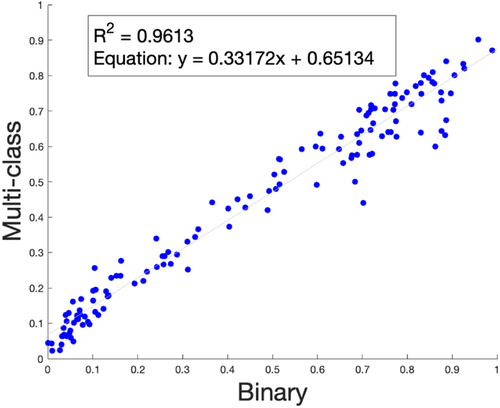
In our comparison of our binary classification model with our multi-class model, we evaluated predicted cell counts with the ground truth (established from manual counting) across sub-images and found a low average error (e < 0.1) across samples (raw data not shown). Furthermore, when we plotted the percentage of empty lacunae predicted by the multi-class cell classifier (Y-axis) against that predicted by the binary cell classifier (X-axis), the predictions for empty lacunae percentage across N = 135 images remained comparable for both models (Figure 9, R = 0.98). This suggests that the newly identified pyknotic cells (with malformed or peripherally displaced nuclei) are a subset of the previous second class, “Osteocyte,” which included all cells with a visible nucleus.
4 DISCUSSION
Although we used a model of steroid-associated ONFH in rabbits as a model of early stage ONFH in humans, the ideal animal model of ONFH has not yet been established. In addition, the pathological criteria for ONFH have not been standardized.19 The most commonly used criteria for steroid-associated ONFH in rabbits are diffuse empty lacunae or pyknotic osteocytes within the bone trabeculae coupled with surrounding bone marrow cell necrosis.12 Others have reported enlarged fat cells in the absence of hematopoietic cells within the bone marrow, as well as pyknotic nuclei, or malformed osteocytes with peripherally displaced nuclei, concentrated in the subchondral bone of corticosteroid-treated rabbits.20 Healthy rabbits without any corticosteroid treatments typically have hematopoietic cells and few empty lacunae within the bone marrow, and a majority of normal osteocytes with round or oval nuclei in the subchondral bone.20 In our studies, in which we took randomly sampled images of the subchondral region of the femoral head, we saw diffuse empty lacunae and pyknotic nuclei in all images (Figure S1). Hence, we concluded that all rabbits in our studies exhibited osteonecrotic changes in the femoral head after corticosteroid injection.
Our decision to shift from using the MATLAB Image Processing Toolbox to using a deep convolutional neural network was driven by our desire to automate the histology image cell quantification process while optimizing for accuracy. Although other studies have reported success in tuning image thresholds using MATLAB algorithms for immunohistochemistry analyses,21 the variations in image color and contrast between our samples made it difficult to consistently and accurately assess the number of osteocytes and empty lacunae. We were surprised to find that only a small subset (N = 27) of the full image data set (N = 135) was needed to train a neural network to obtain a robust binary cell classifier that accurately (adjusted R2 > 0.95) identified our features of interest. Typically, a training set size of at least N = 200 is recommended for accurate object detection and classification (defined as above a 95% recognition rate), and many medical imaging applications require training of upwards of N = 1000 images with careful annotation by trained professionals to develop a robust classifier.22-24 To our knowledge, this is the first application of a convolutional neural network to quantify the percentage of empty lacunae for evaluation of the treatment efficacy of early stage avascular necrosis.
The methods detailed in this study can be extended to automate other histology and immunohistochemistry image analysis applications that require significant time and expertise, such as the manual counting of multiple cell lines or stained blood vessels. However, there are still several limitations of this study. Although we were able to develop an automated system that accurately detects, classifies, and enumerates osteocytes and empty lacunae in new histological images, training a robust cell classifier takes a significant amount of overhead time and iteration, and it may not be the most time-efficient method for analyzing smaller datasets. Furthermore, due to the lack of standardization for the pathology criteria for ONFH, and because we wanted to demonstrate the feasibility of developing an osteonecrosis classifier using convolutional neural networks, our model was trained with image examples from H&E-stained images, specifically for ONFH tissue samples from a rabbit disease model, and our training data did not include other common staining and tissue types.
While some broader multiclass object detection classifiers exist, these are products of millions of training examples that are typically generic images of objects of interest (cat, house, etc.). In our case, we aimed to develop a classification system for a specific application, early stage osteonecrosis, and in this proof of concept study, we narrowed our training set to a specific species, rabbits, to evaluate the efficacy of our model without the need to label and train millions of training examples from different species. It is also important to note that focusing on the percentage of empty lacunae within subchondral regions of the femoral head does not fully represent all early signs of osteonecrosis, which may also include pyknotic osteocytes and apoptotic osteocytes within the subchondral region and enlarged fat cells in the extraskeletal regions such as the bone marrow. While we understand the limitations of our binary classifier model, which only distinguishes between osteocytes and empty lacunae, thereby categorizing all cells with a visible nucleus as osteocytes, the methodology highlighted in this study can still be used to develop a new osteonecrosis classifier with more classes and training examples.
To that end, we updated our model to include a classification of pyknotic nuclei. To do this, we experimentally added a small number of training examples for a third class, pyknotic osteocytes, into our previously binary model with two classes and systematically established the ground truth via independent manual counting by several experienced researchers (Figure S3). In our study, we found that the multi-class classifier also accurately distinguishes among three classes of cells when compared with manually counted results (Figure S4, raw data not shown). Furthermore, when we evaluated the percentage of empty lacunae across our binary classification model and our multi-class model, we found a comparable percentage of empty lacunae, suggesting that newly identified pyknotic cells were distinguished from the previously classified “Osteocyte” group in the binary model (Figure 9).
Although we saw surprisingly accurate results from our binary classifier by training a small subset of data (N = 27, n = 135), in the future, we plan to further improve the robustness of our cell classifier by including other staining conditions, species, and cell types. Finally, we did not compare our results with other free or commercially available machine learning software, and in the future, we can further refine our algorithms by implementing additional resources from the OpenCV library and other advanced image preprocessing tools. Despite these limitations, we believe that our results and methodology in developing this osteonecrosis cell classification system using deep convolutional neural networks will greatly benefit the medical imaging communities and those interested in avascular necrosis and help to expedite the analysis of histological images for researchers in these fields.
5 CONCLUSIONS
We have successfully developed an automated cell counting platform utilizing the power of AI and convolutional neural networks, which have significantly reduced the manual time and effort of counting cells in our histological analyses of treatments for ONFH. The methods detailed in this study can be translated to automate other fields of image analysis that require significant time and expertise, such as the manual counting of blood vessels and other cell types. It is worth noting that the algorithms and methodology highlighted in this manuscript are not file type specific, thus conducive to use with many different image acquisition methods, and can easily be translated to use in other staining protocols and species with training and calibration. These methods would also be valid when building a larger model with more training examples and classes, as illustrated by our multi-class model. In future work, we plan to build an even more robust osteonecrosis cell classifier using training data from multiple species and publish the classification system and methodology online, so that other researchers can access and use these tools for a variety of studies across species.
ACKNOWLEDGMENTS
This study was funded through the financial support of NIAMS grants R01AR057837, U01AR069395, R01AR072613, R01AR074458, DoD grant W81XWH-20-1-0343, and the NSF GRFP Fellowship.
AUTHOR CONTRIBUTIONS
Elaine Lui drafted the manuscript and conducted image preprocessing, annotations, neural network training, data analysis, and image quantification. Masahiro Maruyama and Roberto A. Guzman performed histologic sectioning, staining, and imaging, and conducted independent manual cell counting. Seyedsina Moeinzadeh developed materials used for treatment groups in rabbit studies. Chi-Chun Pan developed the first implementation of the MATLAB multi-cell counting algorithm. Alexa K. Pius, Madison S. V. Quig, and Laurel E. Wong analyzed and labeled histological images containing the pyknotic nuclei class. Stuart B. Goodman and Yunzhi P. Yang advised on this study and performed manuscript revisions. All authors have read and approved this manuscript for final submission.


