Simultaneous total intracranial volume and posterior fossa volume estimation using multi-atlas label fusion
Abstract
Total intracranial volume (TICV) is an essential covariate in brain volumetric analyses. The prevalent brain imaging software packages provide automatic TICV estimates. FreeSurfer and FSL estimate TICV using a scaling factor while SPM12 accumulates probabilities of brain tissues. None of the three provide explicit skull/CSF boundary (SCB) since it is challenging to distinguish these dark structures in a T1-weighted image. However, explicit SCB not only leads to a natural way of obtaining TICV (i.e., counting voxels inside the skull) but also allows sub-definition of TICV, for example, the posterior fossa volume (PFV). In this article, they proposed to use multi-atlas label fusion to obtain TICV and PFV simultaneously. The main contributions are: (1) TICV and PFV are simultaneously obtained with explicit SCB from a single T1-weighted image. (2) TICV and PFV labels are added to the widely used BrainCOLOR atlases. (3) Detailed mathematical derivation of non-local spatial STAPLE (NLSS) label fusion is presented. As the skull is clearly distinguished in CT images, we use a semi-manual procedure to obtain atlases with TICV and PFV labels using 20 subjects who both have a MR and CT scan. The proposed method provides simultaneous TICV and PFV estimation while achieving more accurate TICV estimation compared with FreeSurfer, FSL, SPM12, and the previously proposed STAPLE based approach. The newly developed TICV and PFV labels for the OASIS BrainCOLOR atlases provide acceptable performance, which enables simultaneous TICV and PFV estimation during whole brain segmentation. The NLSS method and the new atlases have been made freely available. Hum Brain Mapp 38:599–616, 2017. © 2016 Wiley Periodicals, Inc.
INTRODUCTION
Total intracranial volume (TICV), the volume inside the brain cranium, is the total volume of gray matter (GM), white matter (WM), cerebrospinal fluid (CSF), and meninges [Mathalon et al., 1993]. In volumetric analyses, many inter-subject differences can be explained by differences in head size [Barnes et al., 2010]. To reduce variability, TICV has been widely used as a covariate in regional and whole brain volumetric analyses [Barnes et al., 2010; Farias et al., 2012; Nordenskjold et al., 2013; Peelle et al., 2012; Perlaki et al., 2014; Westman et al., 2013; Whitwell et al., 2001]. Compared with whole brain volume (WBV) [Smith, 2002], TICV is often preferred since it provides an estimation of premorbid brain size [Davis and Wright, 1977; Perneczky et al., 2010].
Manual delineation of the cranial vault is the gold standard for measuring TICV from magnetic resonance (MR) images [Whitwell et al., 2001]. However, this labor-intensive and time-consuming procedure is impractical on large cohort. As a result, automatic TICV estimation methods are appealing. One family of methods directly applies the automatic skull-stripping techniques to TICV estimation for particular imaging modalities. In MRI, skull is dark while CSF is bright in some modalities [e.g., T2-weighted (T2w) and proton density (PD)]. Therefore, the brighter CSF and brain tissues are able to be segmented from the darker skull using skull-stripping, and the total volume of the CSF and brain tissues are used as TICV. For instance, the brain extraction tool (BET) and the brain surface extractor (BSE) achieved accurate TICV estimation using PD images [Hartley et al., 2006]. However, both skull and CSF are dark in other modalities [e.g., T1-weighted (T1w)], in which the skull-stripping techniques typically yield less accurate TICV estimations because of the low contrast between the CSF and skull. To derive accurate TICV estimation on such MR modalities, a number of approaches have been developed and evaluated [Aguilar et al., 2015; Ananth et al., 2014; Ashburner and Friston, 2005; Buckner et al., 2004; Driscoll et al., 2009; Hansen et al., 2015; Keihaninejad et al., 2010; Lemieux et al., 2003; Pengas et al., 2009; Smith et al., 2004]. Among these methods, three of the most prevalent are integrated in FreeSurfer (FS) [Dale et al., 1999], FMRIB Software Library (FSL) [Smith et al., 2004], and Statistical Parametric Mapping (SPM12). In FreeSurfer, the estimated TIV (eTIV) tool estimates TICV by investigating the affine transformation between target image and template [Buckner et al., 2004]. The idea is that the TICV volume is correlated with the determinant of the transform matrix (called “scaling factor”), which aligns a target image with a template. SIENAX, part of FSL, also provides a volumetric scaling factor as a normalization for head size [Fein et al., 2004]. This scaling factor is the determinant of scaling matrix from affine registration, which rescales the target image's skull to the template's skull [Smith et al., 2002]. Therefore, FreeSurfer and FSL do not provide explicit skull/CSF boundaries (SCB) when estimating TICV. SPM provides two different approaches for TICV estimation (e.g., implemented in SPM5 and SPM8). The first approach, called the reverse brain mask (RBM) method, non-rigidly registers a TICV mask from template space to individual space [Boyes et al., 2006; Keihaninejad et al., 2010]. The second approach accumulates the tissue probabilities of GM, WM, and CSF in standard space using the “New Segment” toolbox [Ashburner and Friston, 2005; Weiskopf et al., 2011]. The first approach provides a TICV mask in individual space; however, the second method produces more accurate TICV estimations [Ridgway et al., 2011]. More recently, the newly released SPM12 provides a new “Tissue Volumes” toolbox, which combines the advantages from two previous approaches in a unified framework [Malone et al., 2015]. As a result, SPM12 achieves superior TICV estimations compared with previous SPM versions [Malone et al., 2015]. However, the TICV value and the related SCB are provided in standard space by SPM12 rather than in individual space. Extra efforts from the user side are required if the users want to achieve consistent TICV value and SCB in individual space.
FreeSurfer, FSL and SPM12 are three of the most well validated and widely accepted TICV estimation software packages. However, none of them estimate TICV by counting the voxels inside skull (or SCB), which is a natural way of calculating TICV. The reason is that it is difficult to obtain adequate intensity contrast between skull and CSF in MR T1-weighted (T1w) images (assuming that the thickness of dura is negligible). To obtain the SCB, multispectral MR data [e.g., T2-weighted (T2w), proton density (PD)], with more clear skull evidence, have been combined with T1w images in TICV estimation [Hansen et al., 2015; Keihaninejad et al., 2010; Pengas et al., 2009; Whitwell et al., 2001]. However, it is still essential to measure TICV with explicit SCB using a single T1w image since: (1) T2w and PD images are not available in all datasets and T1w images are commonly available structural MR sequences. (2) TICV estimation with SCB not only leads to a natural way of obtaining TICV (count voxels inside skull) but also allows us to calculate sub-region volumes, for example, posterior fossa volume (PFV), which is essential in investigating cerebellum development, for example, [Badie et al., 1995; Nyland and Krogness, 1978; Sgouros et al., 2006].
TICV estimation using STAPLE label fusion [Warfield et al., 2004] has been proposed to derive SCB using a single T1w image [Schaerer et al., 2012]. However, the STAPLE label fusion algorithm has shown limitations [Van Leemput and Sabuncu, 2014], which have led to extensions of STAPLE [Akhondi-Asl et al., 2014; Asman and Landman, 2011, 2012, 2013, 2014; Commowick and Warfield, 2010; Landman et al., 2012; Rohlfing et al., 2003a, 2003b; Shen et al., 2015]. Recently, an improved method called Non-local Spatial STAPLE (NLSS) label fusion, a combination of Spatial STAPLE [Asman and Landman, 2012] and Non-local STAPLE (NLS) [Asman and Landman, 2013], has shown advantages over STAPLE, Spatial STAPLE and NLS in brain segmentation [Asman et al., 2015; Asman and Landman, 2014; Huo et al., 2015, 2016a, 2016b], optic nerve segmentation [Harrigan et al., 2014, 2015, 2016; Panda et al., 2014] and spinal cord segmentation [Asman et al., 2014]. Therefore, using NLSS in TICV estimation is promising as it takes both spatial varying performance and non-local intensity correspondence into account. Although the NLSS method has been successfully applied in different applications, its mathematical derivation has not been published yet, which hinders other researchers seeking to implement and use NLSS methods.
In this article, we proposed to use NLSS approach to estimate TICV and PFV simultaneously from a single MR T1w image. The main contributions of this work are: (1) TICV and PFV are simultaneously obtained with explicit SCB. (2) We develop TICV and PFV labels for 45 images of the widely used OASIS dataset under BrainCOLOR protocol [Klein et al., 2010; Landman and Warfield, 2012)] and make a subset freely available online (https://masi.vuse.vanderbilt.edu/index.php/TICV_BC2atlases). (3) This the first journal appearance of NLSS method with detailed mathematical derivation. In the multi-atlas segmentation framework, the pairs of T1w images and TICV labels (atlases) are essential [Iglesias and Sabuncu, 2015]. Normally, atlases are obtained by labor-intensive manual tracing. However, since skull has much higher Hounsfield unit (HU) than other brain tissues [Feeman, 2010], we speed up the atlas generation using a semi-manual strategy to obtain TICV and PFV labels using a dataset with 20 paired MR and CT images. Then, the TICV and PFV labels are propagated to the BrainCOLOR atlases [Klein et al., 2010; Landman and Warfield, 2012]) by deploying NLSS multi-atlas segmentation. From leave-one-out evaluations and reproducibility analyses, the NLSS TICV estimation method demonstrates its advantages compared with FreeSurfer, FSL, SPM12, and a previously proposed STAPLE TICV estimation approach. The new TICV and PFV labels in OASIS BrainCOLOR atlases provide acceptable performance, which enables simultaneous whole brain segmentation as well as TICV and PFV estimation without conducting additional time-consuming non-rigid registrations. Moreover, NLSS tool is publically available as open source software through the JIST software package (http://www.nitrc.org/projects/jist/) [Li et al., 2012; Lucas et al., 2010].
THEORY
The derivation of NLSS closely follows Spatial STAPLE [Asman and Landman, 2012] and NLS [Asman and Landman, 2013], which use Expectation-Maximization (EM) framework [Dempster et al., 1977; McLachlan and Krishnan, 2007]. The majority of the derivations of STAPLE (section “STAPLE”), Spatial STAPLE (section “Spatial STAPLE”), and Non-Local STAPLE (section “Non-local STAPLE”) are left to their original works, but they are described briefly in this work. The notation follows STAPLE [Warfield et al., 2004].
Problem Definition
A target gray-level image with
 voxels is represented as
 . The corresponding latent true segmentation for the target image is given by
 , where
 represents
 possible labels for a given voxel
 (
(
 ). Since T is unknown, the labels for the target image are estimated using
 pairs of atlases with intensity values
 and label decisions
 . In STAPLE family of approaches, the label fusion problem is regarded as a probabilistic estimation of hidden true segmentation based on the performance of multiple atlases. The performance parameter
 indicates the probability that observed label is
 given that the true label is
 for atlas
 (
(
 ). All
 , can be written as a matrix
 , called performance parameters. The
 indicates each
 satisfies
 .
.
STAPLE
 , such that they maximize the complete log-likelihood
 (1)
(1) and the unobserved latent true labels
 . Since
 is not available, the performance parameters are estimated through EM framework. In the E-step, the weight variables
 are derived from
 , where
 represents the probability that the true label of voxel
 is
is
 at iteration
 given
given
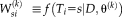 . Applying Bayes' rule and the assumed conditional independence between atlases,
 for a particular voxel and label is given by
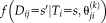
 (2)
(2) is the prior probability that label
 is the true label at
 and will be discussed in section “Non-local Spatial STAPLE.”
 represents all existing labels while
 represents all atlases. Using
 as the simplified expression of
 , the Eq. 2 can be rewritten as
 (3)
(3)The denominator is the partition function to force
 .
.
 as
as
 (4)
(4) (5)
(5) and
and
 . This process iteratively solves for the true data likelihood in the E-Step and updates the performance parameters in the M-step.
Spatial STAPLE
 , are calculated at each voxel [Asman and Landman, 2012]. The parameters are given by
 , which correspond to performance parameters defined voxel-wise instead of globally. As a result, the E-step in Spatial STAPLE is given by
 (6)
(6) is the simplified expression of
 . The M-step follows the derivation of STAPLE, but since the degrees of freedom are a factor of
 higher than STAPLE, two extra extensions are included to account for the increased complexity. First, the performance parameters are binned over small pooling regions instead of a strictly voxel-wise derivation. Following [Asman and Landman, 2012], this is implemented by defining spatial pooling regions
 , where
 is the index of the bin which voxel
 is contained in. Second, the performance is augmented by a non-parametric prior
 on the performance following Asman and Landman [2012] and Landman et al. [2012]. This augmentation improves the stability of the performance parameters. Thus, the M-step is given by
 (7)
(7) .
.
 is a weighting parameter depends on the size of pooling region
 , which balances the prior and the updated probability. We derive
 using the same definition as [Asman and Landman, 2012].
Non-Local STAPLE
 and target image
 into the STAPLE framework using a patch-based non-local correspondence manner [Asman and Landman, 2013]. Patch-based non-local correspondence was initially introduced to account for registration inaccuracy [Coupé et al., 2011]. NLS incorporates patch-based non-local correspondence into the STAPLE framework as follows. The E-step is given by
 (8)
(8) is a search neighborhood around voxel
 and
and
 is the non-local weighting between voxel
 in the target image at voxel
 on the
 atlas, within the search parameter
 .
.
 is given by
 (9)
(9) is the set of intensities within its patch neighborhood. In this definition,
 is the L2-norm between the atlas patch centered at
 and the target patch centered at
 ,
,
 is the Euclidean distance in physical space between
 and
and
 ,
,
 and
and
 are the standard deviations for the intensity and distance weights, respectively, and
 normalizes
 to be a valid probability distribution for each atlas and target voxel. The M-step for Non-Local STAPLE is
 (10)
(10)Non-Local Spatial STAPLE
 (11)
(11)In the NLSS algorithm,
 is spatially varying as in Spatial STAPLE and non-local correspondence is used to account for registration errors.
NLSS E-step
 (12)
(12) (13)
(13)This derivation incorporates both the spatially varying performance parameters derived in Spatial STAPLE and the non-local correspondence derived in Non-local STAPLE.
NLSS M-step
 is used to update
 by maximizing the expectation of the log likelihood function as
 (14)
(14) Multiplier [Bellman, 1956] with constrain
 and setting the derivative equal to zero this becomes
 (15)
(15) (16)
(16) is introduced for computational and stability concerns [Asman and Landman, 2012]. The prior can be derived from a number of approaches (e.g., STAPLE [Warfield et al., 2004], Majority Vote, Locally Weighted Vote [Sabuncu et al., 2010], etc.). In our NLSS implementation, the Majority Vote while ignoring “consensus voxels” (i.e., voxels where all raters agree) is employed as default method [Rohlfing et al., 2004]. This method ignores the consensus voxels when constructing the performance level parameters. Then, the final stable version of Eq. 16 is reformulated to
 (17)
(17) is a weighting parameter depends on the size of pooling region
 , which balances the prior and the updated probability. We derive
 and
and
 using the same way as [Asman and Landman, 2012].
Notice that the Eq. 16 is the theoretical expression of M-step in the EM framework while the Eq. 17 is an approximate maximizer for computational and stability concerns. The implementations of both cases have been provided in the publically available open-source code, which enable the users to switch from each other by controlling
 . In practice, the Eq. 17 typically provides better performance than Eq. 16. Therefore, the implementation of Eq. 17 is the default setting in NLSS open-source code.
Initialization, parameters, and detection of convergence
 in NLSS is initialized using the weak log-odds majority vote [Sabuncu et al., 2010]. The performance parameters are typically initialized assuming each atlas has high performance as
 (18)
(18)The search neighborhood
 and the patch neighborhood
 are the two key parameters in non-local search model. The sensitivity of
 and
and
 in NLSS is evaluated in Supporting Information Section S-1 (Supporting Information Fig. S1). In all presented experiments, the search neighborhood
 was set to
 voxels search window centered at a target voxel while the patch neighborhood
 was empirically set to
 voxels. The two standard deviation parameters
 and
and
 in Eq. 7 were empirically set to 0.1 and 1.5, respectively. The algorithm is iterated until the trace of the difference of confusions matrices between iterations is small, typically less than
 .
.
METHOD
This section first introduces a semi-manual method to establish atlases with TICV and PFV labels (section “Semi-Manual Segmentations and Semi-Manual Atlases”). Second, the multi-atlas segmentation framework using NLSS label fusion is demonstrated (section “NLSS Multi-atlas framework”). Third, the procedure of generating TICV and PFV labels for the BrainCOLOR (BC) atlases is introduced (section “TICV and PFV labels for OASIS BrainCOLOR atlases”). Last, the statistical analysis methods used in this work are introduced (section “Statistical Analysis”).
Semi-Manual Segmentations and Semi-Manual Atlases
We start by automatic skull labeling using CT images, then obtain TICV labels (voxels inside brain skull), and finally propagate labels to MR images using rigid registration. The procedure of automatically generating TICV atlas (Fig. 1) is inspired by the recent work [Aguilar et al., 2015]. Briefly, each CT image is aligned to MR image using rigid registration [Ourselin et al., 2001] (Fig. 1a). Then, the skull masks are obtained from CT images, whose voxel values are greater than 300 HU [Sjolund et al., 2014] (Fig. 1b). Then, a 3D closing morphological operation (a dilation followed by an erosion) followed by neck removal [Segonne et al., 2004] is applied on the skull mask to obtain the binary skull label. The closing morphological operation fills the holes in the skull, and the inner side of the filled skull provides the SCB (Fig. 1c).

Semi-manual pipeline of establishing atlases. First, the TICV label is obtained by applying a threshold, morphological operations and the level set method on CT images. Then, the TICV label is propagated to MR image space and the reference PFV label are provided by merging TICV label and the automatic whole brain segmentation. Finally, the semi-manual atlases are obtained by conducting manual refinement on the reference labels. [Color figure can be viewed at wileyonlinelibrary.com]
The TICV segmentation is the region inside the SCB. However, the SCB is not a closed surface (e.g., the foramen magnum in the occipital bone). Such opening regions make it difficult to derive the TICV segmentation by only using morphological operations. To deal with the opening regions automatically, Topology-preserving Geometric Deformable Model (TGDM) [Han et al., 2003] with gradient vector flow (GVF) field [Xu and Prince, 1998] is employed. The Standard Geometric Deformable Model (SGDM) has been widely used in image segmentation due to its parameterization independence and ease of implementation. However, topological flexibility of SGDM is not always desired in medical image segmentation especially when the number of components has been known and must be preserved. Based on our anatomical prior knowledge, the TICV segmentation should only contain one component (one contour surface). Therefore, the TGDM framework is employed to keep such topology. In its implementation, the level set contour of TGDM is moved by the gradient vector flow (GVF) field [Xu and Prince, 1998]. The advantage of GVF field is that it forces the contour toward skull and has close to zero force at the opening regions. We also apply a curvature force [Han et al., 2003] to keep the surface smooth at the opening regions. Using TGDM, the non-skull voxels inside zero level set are labeled as TICV segmentation. Such segmentation has a smooth boundary at the opening regions. By copying the labels from the registered CT images voxel-by-voxel, we obtain skull and TICV labels on MR images (Fig. 1d).
Then, we label posterior fossa within the TICV labels. Instead of doing complete manual delineation, a rough automatic segmentation is provided as the reference labels to accelerate the procedure. Briefly, we start with a NLSS multi-atlas segmentation to obtain the whole brain segmentations (133 labels) for each MR image under BrainCOLOR protocol [Klein et al., 2010; Landman and Warfield, 2012] (Fig. 1f). Then, we group the cerebrum regions (above tentorium cerebelli) together, which excludes the CSF and tissues in posterior fossa tissues (cerebellum and brainstem) (Fig. 1g). A closing morphological operation is conducted to obtain the reference labels (Fig. 1h and 1j), which indicates the rough location of posterior fossa. Finally, a manual refinement step is conducted by an experienced graduate student to correct the inaccurate voxels in the reference labels and obtain the final PFV labels (Fig. 1j). Using this semi-manual pipeline, we obtain the 20 atlases consist of both T1w images and labels (posterior fossa, cerebrum, and background). The TICV is the sum of posterior fossa and cerebrum.
NLSS Multi-Atlas Framework
We use a canonical multi-atlas segmentation framework which contains registration, atlas selection, label propagation, and label fusion [Iglesias and Sabuncu, 2015]. Briefly, the target image is first corrected by a N4 bias field correction [Tustison et al., 2010] and then affinely registered [Ourselin et al., 2001] to the MNI305 atlas [Evans et al., 1993]. Practically, using 10–20 atlases are sufficient to achieve accurate whole brain segmentation [Aljabar et al., 2009]. Empirically, the 15 closest atlases with smallest Euclidian distance to the target image on PCA manifold are chosen if total number of available atlases is greater than 15 [Asman et al., 2015]. Then, the 15 selected atlases are then non-rigidly registered to the target image [Avants et al., 2008]. For non-rigid registration, we use symmetric image normalization (SyN), with a cross correlation similarity metric convergence threshold of
 and convergence window size of 15, provided by the Advanced Normalization Tools (ANTs) software [Avants et al., 2008]. Finally, the proposed NLSS label fusion is used to combine the labels from each atlas to the target image. After multi-atlas labeling, each voxel is assigned to one of the labels.
TICV and PFV Labels for OASIS BrainCOLOR Atlases
Using the semi-manual strategy described in section “Semi-manual Segmentations and Semi-manual Atlases,” Researchers are able to reconstruct semi-manual atlases using their own data. However, the paired MR and CT images are not typically available, especially when people want to derive both TICV and PFV labels as well as whole brain segmentation simultaneously (e.g., 133 labels in BrainCOLOR protocol). Therefore, we propagate the TICV and PFV labels from semi-manual atlases to the BrianCOLOR atlases [Klein et al., 2010; Landman and Warfield, 2012], which consist of 45 OASIS images [Marcus et al., 2007]. We have made a subset of the new BrainCOLOR atlases freely available online to facilitate the community.
Briefly, the semi-manual atlases (Fig. 2b) are employed to segment 45 OASIS T1w images using the NLSS multi-atlas segmentation (Fig. 2c). Then, the TICV and PFV labels are derived for the OASIS dataset, which are referred as BrainCOLOR1 (BC1) atlases. Then, the BrainCOLOR2 (BC2) atlases are derived by combining TICV and PFV labels with 133 original labels in BrainCOLOR atlases. Note that if the original manual labels conflict with the TICV or PFV definition in BC1 atlases, we keep the original labels in BC2. Finally, The BrainCOLOR3 (BC3) atlases are obtained by merging the TICV and PFV labels in BC2 atlases.

BC1, BC2, and BC3 atlases are obtained by adding TICV and PFV labels. (a) 20 paired MR-CT images are used to generate (b) semi-manual atlases. Then the NLSS multi-atlas segmentation is conducted on (c) T1w images 45 OASIS images in BrainCOLOR (BC) atlases to achieve TICV and PFV labels. (d) The first automatic segmentation results are referred as BC1 atlases. (e) Then the original 133 labels from BC are merged with BC1 atlases by keeping the BC labels if conflictions happen. The merged BC2 atlases contain 136 labels including the TICV, PFV, and BC labels. (f) The 136 labels are merged back to 4 labels to resolve conflicts and form the BC3 atlases. A subset of BC2 atlases have been made freely available online to facilitate other researchers. We compare the performance of BC1, BC2 and BC3 atlases as well as semi-manual atlases in section “Data and Results.” [Color figure can be viewed at wileyonlinelibrary.com]
Statistical Analysis
 (19)
(19) (20)
(20) and
and
 represent any two binary volumes that need to be compared and
 represents the volume of regions. Dice values evaluate the overlap between regions
 and
and
 which takes both volumetric and spatial information into account. Moreover, the mean surface distance (MSD) between
 and
and
 is also employed to measure the average surface distance between binary volumes.
 (21)
(21)After obtaining the previous metrics, the Wilcoxon signed rank test [Wilcoxon, 1945] is used for statistical analyses. All claims of statistically significance in this article are made using the Wilcoxon signed rank test for P < 0.05.
DATA AND RESULTS
Accuracy Test
Twenty subjects, with both MR and CT images from the deep-brain stimulation (DBS) project, were employed to evaluate the accuracy of TICV and PFV estimation. The MR images were 3D T1w volumes with 256
 256
256
 190 voxels, which have 1
 1
1
 1 mm resolution. The CT images were acquired with pixel size = 0.49 mm, slice thickness = 0.625 mm and FOV = 250
 250
250
 190 mm. From these paired MR-CT images, 20 semi-manual atlases (MR T1w images and labels) were generated using the semi-manual method described in section “Semi-manual Segmentations and Semi-manual Atlases.” Note that the CT images were only used in generating semi-manual atlases, but were not used in the evaluations.
First, FreeSurfer (FS), FSL, and SPM12 were deployed on the 20 T1w MR images to estimate the TICV results. Then, the NLSS multi-atlas framework was deployed on the same dataset using leave-one-out strategy. In each leave-one-out test, other 19 atlases were used as candidate atlases, which ensured the independence to the testing image. The linear relationship between the estimated TICV results and true TICV volumes (semi-manual atlases) were evaluated by linear regressions (Fig. 3). The linear relationship between the estimated TICV results and with the true TICV volumes (semi-manual atlases) were evaluated by linear regressions (Fig. 3). The
 coefficient of determination was provided to indicate how strong the linearity was between measurements, where the higher
 indicated the stronger linearity. From the results, the NLSS TICV estimation achieved the largest
 values (
 = 0.970) to the semi-manual segmentations while FSL had the lowest
 . NLSS TICV estimation also had
 = 0.942 to FreeSurfer and
 = 0.956 to SPM12. The lower right box plot indicated the ASIM scores for different methods compared with semi-manual segmentation. NLSS TICV had significant higher ASIM scores than FreeSurfer and SPM12. The ASIM score for FSL was not shown since it only provided scaling factors rather than volumetric values.

(a) Scatter plots comparing FreeSurfer, FSL, SPM12, and NLSS on TICV estimation. In the first column, different automatic methods are compared with semi-manual segmentations by plotting the TICV volumes with a red line of best fit and NLSS method using semi-manual atlases achieves latest R2 = 0.970. The remaining columns show the scatter plots between automatic methods. NLSS method still achieves large R2 values compared with FreeSurfer, FSL, and SPM12. (b) Box plot of ASIM values between FreeSurfer, SPM12, and NLSS with Semi-manual segmentations. The proposed NLSS (“Ref.”) method achieves significantly higher (“
 ”) ASIM scores than FreeSurfer and SPM12. Since FSL only provides scaling factors rather than TICV volumes, it does not have units in (a) and not shown in (b). [Color figure can be viewed at wileyonlinelibrary.com]
Second, NLSS TICV estimation was compared with the previously proposed STAPLE TICV estimation [Schaerer et al., 2012]. For more complete analyses, we also compared the NLSS estimation with other label fusion approaches such as majority vote (MV), Spatial STAPLE, NLS and joint label fusion (JLF) (Table 1 and 2) using the semi-manual atlases. The JLF [Wang et al., PAMI 2013] approach is the state-of-the-art label fusion method using non-local intensity similarity. In each leave-one-out analyses, the BC1, BC2, and BC3 atlases (on 45 OASIS images) were also generated from the 19 semi-manual atlases (using the method in section “TICV and PFV labels for OASIS BrainCOLOR atlases”). Then these intermediate atlases were also deployed on the target image and their accuracies were compared with semi-manual atlases using the same NLSS multi-atlas framework.
| Atlases | Does not use atlases | Semi-manual | BC1 | BC2 | BC3 | ||||||||
|---|---|---|---|---|---|---|---|---|---|---|---|---|---|
| Methods | FS | FSL | SPM12 | MV | STAPLE | SS | NLS | JLF | NLSS | NLSS | NLSS | NLSS | |
| Corr. | Pearson | 0.954 | 0.923 | 0.953 | 0.959 | 0.957 | 0.960 | 0.969 | 0.985 | 0.985 | 0.965 | 0.963 | 0.964 |
| ICC | 0.836 | N/A | 0.916 | 0.961 | 0.936 | 0.957 | 0.964 | 0.985 | 0.985 | 0.942 | 0.964 | 0.907 | |
| ASIM |
 |
0.941 | N/A | 0.964 | 0.976 | 0.971 | 0.977 | 0.979 | 0.986 | 0.986 | 0.972 | 0.978 | 0.961 |
 |
0.032 | N/A | 0.023 | 0.022 | 0.0285 | 0.024 | 0.024 | 0.014 | 0.015 | 0.026 | 0.020 | 0.028 | |
| Dice |
 |
N/A | N/A | N/A | 0.977 | 0.975 | 0.977 | 0.979 | 0.983 | 0.983 | 0.975 | 0.975 | 0.970 |
 |
N/A | N/A | N/A | 0.008 | 0.01 | 0.008 | 0.008 | 0.005 | 0.006 | 0.008 | 0.006 | 0.009 | |
|
MSD (mm) |
 |
N/A | N/A | N/A | 0.968 | 1.058 | 0.984 | 0.888 | 0.725 | 0.743 | 1.106 | 1.112 | 1.245 |
 |
N/A | N/A | N/A | 0.268 | 0.374 | 0.301 | 0.294 | 0.184 | 0.197 | 0.306 | 0.244 | 0.326 | |
-
“Corr.” means correlation analyses. The bold values indicate the best performance. “N/A” means the values are not available since (1) FSL only provides scaling factors rather than TICV volumes, (2) FreeSurfer (FS), and SPM12 (SPM) do not generate hard TICV segmentation in individual space during the standard default processing. Note: “SS” is Spatial STAPLE. “
 ” is the mean and “
 ” is the standard deviation.
| Atlases | Semi-manual | BC1 | BC2 | BC3 | ||||||
|---|---|---|---|---|---|---|---|---|---|---|
| Methods | MV | STAPLE | SS | NLS | JLF | NLSS | NLSS | NLSS | NLSS | |
| Corr. | Pearson | 0.947 | 0.934 | 0.949 | 0.963 | 0.979 | 0.976 | 0.958 | 0.958 | 0.958 |
| ICC | 0.944 | 0.818 | 0.945 | 0.953 | 0.971 | 0.975 | 0.919 | 0.951 | 0.888 | |
| ASIM |
 |
0.975 | 0.940 | 0.973 | 0.974 | 0.982 | 0.984 | 0.963 | 0.973 | 0.953 |
 |
0.023 | 0.029 | 0.021 | 0.018 | 0.017 | 0.016 | 0.02 | 0.018 | 0.02 | |
| Dice |
 |
0.960 | 0.951 | 0.959 | 0.964 | 0.968 | 0.968 | 0.955 | 0.954 | 0.954 |
 |
0.008 | 0.011 | 0.007 | 0.007 | 0.006 | 0.006 | 0.006 | 0.006 | 0.006 | |
|
MSD (mm) |
 |
0.847 | 1.011 | 0.858 | 0.767 | 0.689 | 0.675 | 0.946 | 0.933 | 0.969 |
 |
0.15 | 0.214 | 0.14 | 0.126 | 0.120 | 0.107 | 0.121 | 0.118 | 0.132 | |
- Please see Table 1 for the descriptions of abbreviations.
Table 1 shown four different metrics of evaluating the accuracy of different TICV measurement approaches: (1) Intraclass correlation (ICC) and Pearson Correlation were used to measure the correlation between different methods and semi-manual segmentations. The two-way random single measure was used as the ICC model [Shrout and Fleiss, 1979]. (2) The ASIM values were used to show the accuracy of TICV volumetric estimation. (3) Dice similarity coefficients were employed to take the spatial information into account upon the ASIM metric. (4) MSD values were also derived to measure the average surface distance between binary segmentations. From Table 1, the family of multi-atlas segmentations (MV, STAPLE, SS, NLS, JLF, and NLSS) obtained higher correlation coefficients than the prevalent FreeSurfer, FSL, and SPM12 approaches. The multi-atlas approaches achieved higher mean and smaller standard deviation (std) on ASIM metric. Within the multi-atlas family, when using the same semi-manual atlases, the NLSS TICV estimation achieved higher scores on correlation coefficients, mean ASIM and mean Dice than previously proposed STABLE TICV estimation. Meanwhile, it had the smaller mean MSD and the lower standard deviation than the STAPLE method. The NLSS estimation was significantly superior to MV, Spatial STAPLE, NLS on both TICV (Table 1I) and PFV (Table 2). The NLSS and JLF had advantages on PFV and TICV respectively. However, the differences between NLSS and JLF were not statistically significant. When comparing the performance between different atlases, the BC1, BC2 and BC3 atlases performed worse than the semi-manual atlases on correlation coefficients, mean ASIM, mean Dice, and mean MSD. However, the correlation coefficients and the mean ASIM values of using BC1, BC2, and BC3 atlases were still higher than FreeSurfer, FSL, and SPM12.
Figures 4-6 show the box plots and the statistical results using Wilcoxon signed rank test. In each figure, the statistical analyses were conducted between the NLSS method using semi-manual atlases (marked as reference “Ref.”) with other approaches or different atlases. If the difference was statistically significant, we marked the method with “*” symbol. Otherwise, we marked the method with not significant “N.S.” Figure 4 shows the ASIM values, which only considered volumetric results for both TICV and PFV segmentations. For TICV estimation, the ASIM of NLSS (semi-manual atlases) was significantly higher than FreeSurfer, SPM12, STAPLE, Spatial STAPLE, and NLS. For PFV estimation, the ASIM of NLSS (semi-manual atlases) was significantly higher than STAPLE, Spatial STAPLE, and NLS. The different performance between NLSS and JLF are not statistically significant. Using the same NLSS method with different atlases, the semi-manual atlases performed significantly better than BC1, BC2, and BC3 atlases in both TICV and PFV volumetric estimation.

Box plots and statistical results on volume accuracy. The statistical analyses were conducted between the proposed NLSS TICV estimation using semi-manual atlases (marked as reference “Ref.”) with other approaches or different atlases. If the difference was statistically significant, we marked the other method with “*” symbol. Otherwise, we marked it as “N.S.”. [Color figure can be viewed at wileyonlinelibrary.com]

Box plots and statistical results on Dice coefficients. The statistical analyses were conducted between the proposed NLSS TICV estimation using semi-manual atlases (marked as reference “Ref.”) with other approaches or different atlases. If the difference was statistically significant, we marked the other method with “*” symbol. Otherwise, we marked it as “N.S.”. [Color figure can be viewed at wileyonlinelibrary.com]

Box plots and statistical results on mean surface distance (MSD). The statistical analyses were conducted between the proposed NLSS TICV estimation using semi-manual atlases (marked as reference “Ref.”) with other approaches or different atlases. If the difference was statistically significant, we marked the other method with “*” symbol. Otherwise, we marked it as “N.S.”. [Color figure can be viewed at wileyonlinelibrary.com]
It is also important to note how the improved accuracy is able to be translated into clinical research benefits. We evaluated the statistical power of detecting a group difference between two simulated clinical cohorts using two-sample t-test at significant level 0.05. The power analyses were shown in the Supporting Information section S-2 (Supporting Information Fig. S2).
Figure 5 employed the Dice similarity coefficients as the metric, which took both volumetric and spatial information into account. Since the TICV and PFV segmentations were not provided by the default processing in FreeSurfer, FSL, and SPM12, we conducted statistical analyses within the multi-atlas family. For both TICV and PFV segmentations, the NLSS using semi-manual atlases achieved the significant higher Dice values than MV, STAPLE, Spatial STAPLE, and NLS. The semi-manual atlases also achieved significant higher Dice values than the BC1, BC2, or BC3 atlases. Figure 6 reflected the statistical analyses on MSD. Again, NLSS using semi-manual atlases had the smaller MSD compared with MV, STAPLE, Spatial STAPLE, and NLS. The performance between NLSS and JLF in Figures 5 and 6 are not statistically significant. To visually check the findings in Figures 5 and 6, Figure 7 shows the qualitative performance of different methods on the same subject. The surfaces of the semi-manual segmentations, which used as reference results, were remarked as red contours. The area of positive error (estimate larger than reference) was the area with green and purple color outside the contours while the negative error (estimate smaller than reference) was colored as white.

Qualitative results comparing multi-atlas segmentation methods with semi-manual segmentation. The red contours represent the spatial location of the semi-manual segmentation. The white color indicates the negative error, in which the estimated segmentation is smaller than the semi-manual reference. The green and purple color outside the red contours indicates the positive error, in which the estimated segmentation is larger than reference. [Color figure can be viewed at wileyonlinelibrary.com]
Reproducibility Test
We employed the publicly available Kirby21 dataset (https://www.nitrc.org/projects/multimodal), which consisted of scan-rescan images on 21 subjects [Landman et al., 2011]. Each subject had two scans with multispectral MR data (e.g., MPRAGE, FLAIR, DIT, etc.) and we used 42 T1w MPRAGE images (with 1
 1
1
 1.2 mm resolution over an FOV of 240
 204
204
 256 mm) in this reproducibility test. Ideally, the TICV and PFV estimations between two scans from the same subject should be close to each other.
Figure 8 demonstrated the reproducibility of different methods on the same 21 pairs of scan-rescan T1w images. We used the ADIFF metric to reflect the ratio of the different volume in the total volume. The results indicated that for both TICV and PFV estimations, all methods achieved small ADIFF values (mostly smaller than 2%).

Volumetric reproducibility analysis of different approaches on scan-rescan T1w images. For all methods, inconsistency of TICV estimation between two scans on the same subject is less than 2%. The statistical analyses were conducted between the proposed NLSS TICV estimation using semi-manual atlases (marked as reference “Ref.”) with other approaches or different atlases. If the difference was statistically significant, we marked the other method with “*” symbol. Otherwise, we marked it as “N.S.” [Color figure can be viewed at wileyonlinelibrary.com]
CONCLUSION AND DISCUSSION
This article proposes the simultaneous TICV and PFV estimation framework using multi-atlas label fusion. Using the NLSS multi-atlas framework, we are able to obtain accurate TICV and PFV estimation simultaneously with explicit boundary between skull and CSF. The mathematical derivation is provided for NLSS. The performance of the proposed method was compared with prevalent FreeSurfer, FSL, and SPM12 methods and the previously proposed STAPLE based TICV estimation. For more complete analyses, the NLSS method is also compared with MV, Spatial STAPLE, NLS, and JLF.
Compared with the FreeSurfer, FSL, SPM12, the proposed NLSS approach achieves significant superior performance in TICV estimation with highest correlation coefficients, mean ASIM, mean Dice and lowest mean MSD (Table 1 and 2, Fig. 3). Compared with other label-fusion methods (Figs. 4-6): (1) NLSS approach achieves statistical better performance in simultaneous TICV and PFV estimation than the previously proposed STAPLE method [Schaerer et al., 2012]. (2) NLSS approach achieves statistical superior performance than MV, Spatial STAPLE, and NLS). (3) For ASIM, Dice, and MSD, the differences between NLSS and JLF are not statistically significant, which means NLSS and JLF are comparable accurate in TICV and PFV estimation. From Table 1 and 2, the JLF has overall better measurements in TICV estimation, while the NLSS has better measurements in PFV estimation. From Figure 8, all methods achieve high reproducibility (ADIFF < 0.2). JLF method achieves statistical smaller ADIFF score than NLSS method on TICV estimation. Overall considering all results, JLF is superior on TICV side while NLSS is superior on PFV side when conducting the simultaneous TICV and PFV estimation.
The accuracy and reproducibility are the two essential aspects when evaluating the performance of TICV estimation. FreeSurfer, FSL, and SPM12 achieves high reproducibility demonstrates that the affine registration and tissue segmentation used in the three methods are reproducible. The superior accuracy and high reproducibility indicate that the multi-atlas based approaches do not compromise on reproducibility while providing more accurate estimations. The multi-atlas labeling approaches not only provided more accurate TICV estimation but also estimated PFV simultaneously (which is not available in FreeSurfer, SPM12, and FSL). The PFV is essential in investigating the clinical conditions of the cerebellum [Badie et al., 1995; Nyland and Krogness, 1978; Sgouros et al., 2006]. In the Supporting Information section S-2, we show that the improvement of accuracy in TICV estimation is able to be translated to greater statistical power on simulated clinical cohorts. The continuing investigation of this work would be on the relationship between the accuracy of TICV estimations and the power of detecting differences between empirical datasets. For instance, we could evaluate the statistical power of detecting the differences of particular metrics (corrected by TICV) between patients and controls using different TICV estimation methods.
We provide new TICV and PFV labels on the widely used 45 OASIS images using BrainCOLOR protocol. The new atlases enable simultaneous BrainCOLOR, TICV and PFV segmentation from only one set of time-consuming non-rigid registration. To evaluate the performance of the new BC1, BC2, and BC3 atlases, we compared them with semi-manual atlases using the same NLSS framework. Using these intermediate atlases, we lost less than 2% of accuracy from ASIM and Dice score and increased the MSD to less than 0.5 mm compared with directly using semi-manual atlases. However, the performances of BC1, BC2, and BC3 atlases are still better than FreeSurfer, FSL and SPM12 (Table 1). Since the BC2 atlases have included original BrainCOLOR labels, we provide a subset of BC2 atlases freely available online to facilitate other researchers (https://masi.vuse.vanderbilt.edu/index.php/TICV_BC2atlases). The T1w MR images of the same OASIS images for BC2 atlases are available via subscription from Neuromorphometrics Inc. (http://www.neuromorphometrics.com/) and the subset of them are freely available from MICCAI 2012 Grand Challenge and Workshop on Multi-Atlas Labeling [Landman and Warfield, 2012] (https://masi.vuse.vanderbilt.edu/workshop2012/).
The semi-manual atlas generation method may be applied on other datasets if paired MR and CT images are available. The rigid registration is used to align CT and MRI images in this study. The registration performance might be affected if huge neck/jaw movements happen in either modality. For such cases, applying a brain mask (masking out neck and jaw) before registration would address the movement issue. The proposed NLSS multi-atlas segmentation framework is flexible in terms of incorporating other regions of interest during TICV estimation. For example, recently, multi-atlas labeling has been used to label brain skull on CT-MRI datasets [Torrado-Carvajal et al., 2016]. In TICV and posterior fossa estimation, we only interested in the accuracy of the inner skull boundary, so we did not seek to fully characterize the cranium. However, it would be interesting to simultaneously provide TICV, PFV and skull labels in the future. The TICV estimation using multi-atlas segmentation is computationally more expensive than using FreeSurfer, FSL and SPM since multiple non-rigid registrations (≈1.5 hours per registration) are conducted for a target image. However, the total length of running time can be reduced by running such independent registrations in parallel. Moreover, the computed registration can be used for other purpose (e.g., segmenting other brain structure, morphometry, manifold learning, etc.).
ACKNOWLEDGMENT
This research was conducted with the support from Intramural Research Program, National Institute on Aging, NIH. This study was also supported in part using the resources of the Advanced Computing Center for Research and Education (ACCRE) at Vanderbilt University, Nashville, TN. The content is solely the responsibility of the authors and does not necessarily represent the official views of the NIH. The authors have no conflict of interest to declare.